© April
2014, Darrell Cox (last updated on
August 31, 2019)
A convolution of the differences of the zeta function zeros with the Möbius function is discussed at zeros. Associated software is at test3 (convolution with Möbius function), mobius, nucheck, primed, table2, test5c (compute probit function), test9a (compute Mertens function), test2n (Dirichlet products and Möbius inversion), interp1, test2g (Fourier transform of modified Riemann spectrum), zero1 (100,000 zeta function zeros), newrat3 (compute Riemann's R(x)), and nugauss (corresponding computations for Gaussian primes). The table of the first 10,000,000 zeta function zeros ("zerob.h") is not included. A 64-bit OS is required to run "test3". A summary of results pertaining to bounds of the Mertens function is given at bounds. Statistical properties of the zeta function zeros and standard uniform distributions are compared at unizeta. A general summary of this article is given at latest. Previous summaries (partially outdated) are at nuriem, newreim, and farreim. Let A(x) denote Σi=1xφ(i) where φ is Euler's totient function and let M(x) denote the Mertens function. A plot of √Σi=1xM([x/i])2, A(x)/√(x(x+1)(2x+1)/6), and |M(x)| versus √x for x=2, 3, 4, ..., 100000 is;
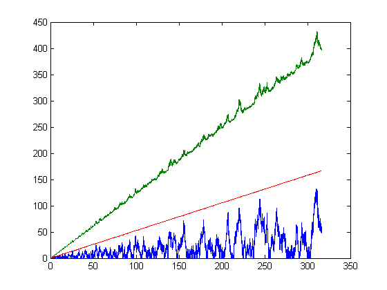
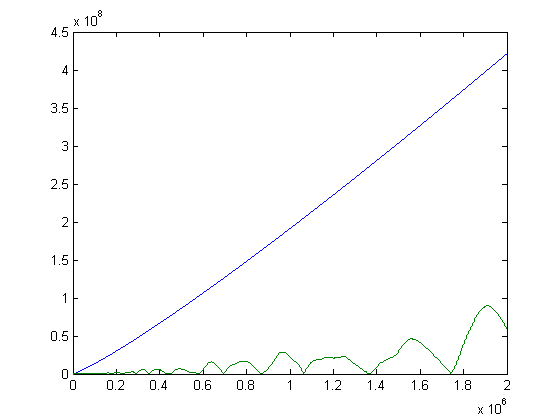
Σi=1xM([x/i])i=A(x) and by the Schwarz inequality A(x)/√(x(x+1)(2x+1)/6) is less than or equal to √Σi=1xM([x/i])2. (The brackets "[ ]" denote the floor function.) A plot of √Σi=1xM([x/i])2 versus √x for x=2, 3, 4, ..., 1000000 is;
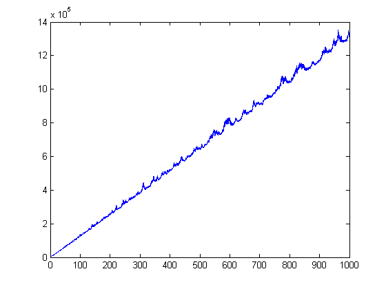
A plot of Σi=1xM([x/i])2 and 8Σi=1xsgn(M([x/i]))-20 versus x for x=2, 3, 4, ..., 300 is;
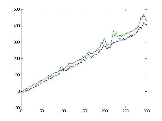
(Note that Σi=1xsgn(M([x/i]))=O(x).) A plot of √Σi=1xM([x/i])2 and √8.7√Σi=1xsgn(M([x/i]))-2 versus x for x=2, 3, 4, ..., 1000 is;
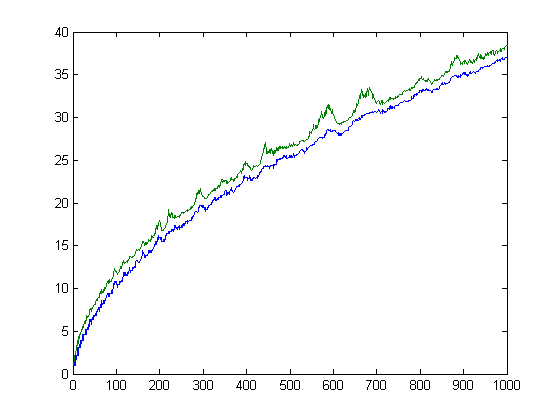
Let k=[x/6] and r=x-6k. Let g(1), g(2), g(3), g(4), and g(5) equal 1, 2, 4, 6, and 11 respectively. If k>0 and r=0, let g(x)=12k+23(k(k-1))/2. If k>0 and r=1, let g(x)=12k+23(k(k-1))/2+7+6(k-1). If k>0 and r=2, let g(x)=12k+23(k(k-1))/2+11+9(k-1). If k>0 and r=3, let g(x)=12k+23(k(k-1))/2+17+13(k-1). If k>0 and r=4, let g(x)=12k+23(k(k-1))/2+22+16(k-1). If k>0 and r=5, let g(x)=12k+23(k(k-1))/2+33+22(k-1). g(x) is an empirically derived lower bound of Σi=1xsgn(M([x/i]))i. A plot of √Σi=1xsgn(M([x/i]))i-√g(x) versus x for x=2, 3, 4, ..., 200 is;
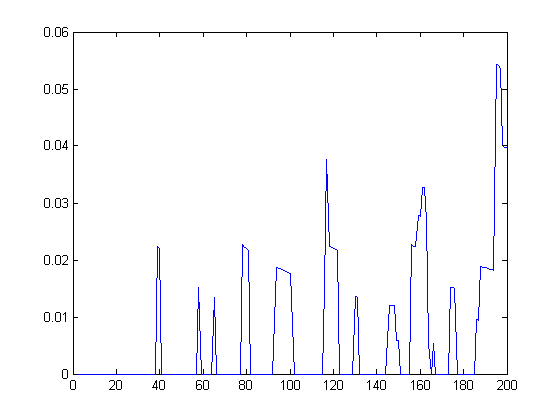
For a linear least-squares fit of √Σi=1xsgn(M([x/i]))i-√g(x) versus x for x=2, 3, 4, ..., 100000, p1=6.103e-5 with a 95% confidence interval of (6.103e-5, 6.104e-5), p2=3.05e-5 with a 95% confidence interval of (-0.0001669, 0.0002279), SSE=25.35, R-square=0.9999, and RMSE=0.01592. A plot with bounding lines having y-intercepts of 0.15 more and 0.15 less and the same slope is;
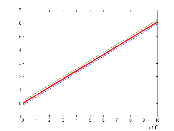
For a linear least-squares fit where x=2, 3, 4, ..., 1000000, p1=6.103e-5 with a 95% confidence interval of (6.103e-5, 6.103e-5), p2=-0.00046 with a 95% confidence interval of (-0.0005797, -0.0003404), SSE=931.5, R-square=1, and RMSE=0.03052. A plot with bounding lines having y-intercepts of 0.8 more and 0.8 less and the same slope is;
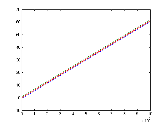
The variation in the √Σi=1xsgn(M([x/i]))i-√g(x) values appears to be slowly increasing. Based on this data, g(x)/√(x(x+1)(2x+1)/6) is a lower bound of √Σi=1x(sgn(M([x/i])))2. (Note that √Σi=1x(sgn(M([x/i])))2=O(x½).) Σi=1xsgn(M([x/i]))i is slightly greater than A(x). For a linear least-squares fit of √Σi=1xM([x/i])i versus x for x=2, 3, 4, ..., 50000, p1=0.5513 with a 95% confidence interval of (0.5513, 0.5513), p2=0.2758 with a 95% confidence interval of (0.2736, 0.2781), SSE=816.9, R-square=1, and RMSE=0.1278. For a linear least-squares fit of √Σi=1xM([x/i])1/3i versus x for x=2, 3, 4, ..., 50000, p1=0.5617 with a 95% confidence interval of (0.5617, 0.5617), p2=0.2809 with a 95% confidence interval of (0.2786, 0.2832), SSE=859, R-square=1, and RMSE=0.1311. For a linear least-squares fit of √Σi=1xM([x/i])1/5i versus x for x=2, 3, 4, ..., 50000, p1=0.5633 with a 95% confidence interval of (0.5633, 0.5633), p2=0.2817 with a 95% confidence interval of (0.2793, 0.284), SSE=890.9, R-square=1, and RMSE=0.1335. For a linear least-squares fit of √Σi=1xM([x/i])1/7i versus x for x=2, 3, 4, ..., 50000, p1=0.5639 with a 95% confidence interval of (0.5639, 0.5639), p2=0.282 with a 95% confidence interval of (0.2796, 0.2843), SSE=905.1, R-square=1, and RMSE=0.1345. For a linear least-squares fit of √Σi=1x sgn(M([x/i]))i versus x for x=2, 3, 4, ..., 50000, p1=0.5653 with a 95% confidence interval of (0.5653, 0.5653), p2=0.2827 with a 95% confidence interval of (0.2803, 0.2851), SSE=942.3, R-square=1, and RMSE=0.1373.
Let d denote the height of a step of the function √Σi=1xsgn(M([x/i]))i. d is less than or equal to 1.0. A histogram of [200d+0.5] for x≤500000 is;
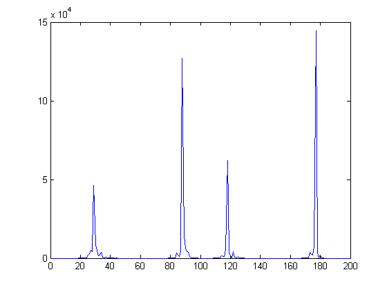
(Two of the expected six step sizes are approximately equal.) Let e denote the height of a step of the function g(x). The bin-by-bin difference in the histograms of [200d+0.5] and [200e+0.5] for x≤1000000 is;
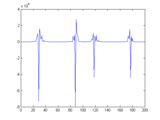
Let d denote the height of a step of the function √Σi=1xM([x/i])i. A histogram of [200d+0.5] for x≤500000 is;
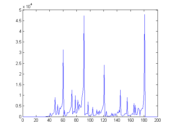
Let d denote the height of a step of the function √Σi=1xM([x/i])1/3i. A histogram of [200d+0.5] for x≤500000 is;
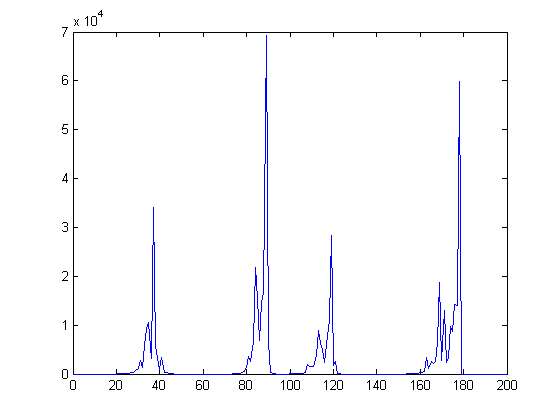
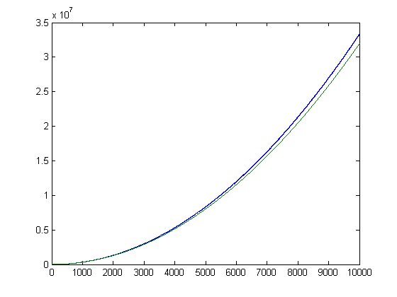
Let h(x) denote Σi=1x(n[x/i]-m[x/i]) where mx denotes the number of fractions before 1/4 and nx denotes the number of fractions between 1/4 and 1/2 in a Farey sequence of order x. (Although 1/4<1/3<1/2, n3 is set to 0 since 1/4 is not in a Farey sequence of order 3.) h(2), h(3), h(4), ..., and h(13) equal 0, 0, 1, 1, 0, 1, 2, 1, 1, 2, 2, and 2 respectively and h(x+12)=h(x)+2 (based on empirical evidence). (The property Σi=1x(m[x/i]-n[x/i]+1/6)=1, 2/3, 1/2, 1/3, 1/6, 0, -1/6, -1/3, or -2/3 is analogous to the property Σi=1xM([x/i])=1 and can be proved similarly. As will be shown, there are infinitely many "Riemann hypotheses" associated with Farey sequences.) 12(h(x))2 is approximately equal to g(x) (for x>270, 12(h(x))2>g(x)). A plot of 12(h(x))2 and g(x) versus x for x=2, 3, 4, ..., 10000 is;
h(x) appears to be a lower bound of Σi=1xsgn(M([x/i])). A plot of Σi=1xsgn(M([x/i]))-h(x) versus x for x=2, 3, 4, ..., 1000 is;
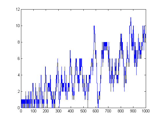
Σi=1xsgn(M([x/i])) equals h(x) in 47 instances. A plot of h(x)-Σi=1xsgn(n[x/i]-m[x/i]) versus x for x=2, 3, 4, ..., 1000 is;
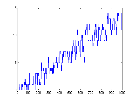
h(x) equals Σi=1xsgn(n[x/i]-m[x/i]) in 56 instances. A plot of Σi=1x(n[x/i]-m[x/i])2-Σi=1xsgn(M([x/i])) versus x for x=2, 3, 4, ..., 300 is;
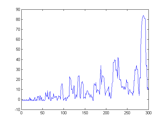
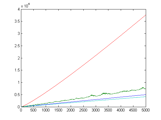
1+Σi=1x(n[x/i]-m[x/i])2 equals Σi=1xsgn(M([x/i])) in 39 instances. Based on empirical evidence, log(x!)≥Σi=1xM([x/i])2≥ψ(x)≥Σi=1x|sgn(M([x/i]))|≥1+Σi=1x(n[x/i]-m[x/i])2 ≥Σi=1xsgn(M([x/i]))≥h(x)≥Σi=1xsgn(n[x/i]-m[x/i]). ψ(x) denotes the second Chebyshev function. Mertens proved that Σi=1xM([x/i])log(i)=ψ(x). Apparently, the log(i) factor is not large enough to give an upper bound of Σi=1xM([x/i])2. Σi=1xM([x/i])log(i)d(i)=log(x!) where d(i) denotes half the number of positive divisors of i. log(x!)=xlog(x)-x+O(log(x)), so this is a likely upper bound of Σi=1xM([x/i])2. (Since log(x) increases more slowly than any positive power of x, this is a better upper bound than x1+ε where ε>0.) A plot of log(x!), Σi=1xM([x/i])2, ψ(x), and Σi=1x|sgn(M([x/i]))| versus x for x=2, 3, 4, ..., 5000 is;
Σi=1xM([x/i])d(i)=x/2. d(i) is half the sum of positive divisors function σ0(i). (Σn=1∞σ0(n)/ns =ζ(s)2 where ζ(s) is the Riemann zeta function.) A plot of Σi=1x(n[x/i]-m[x/i])d(i) versus x for x=2, 3, 4, ..., 10250 is;
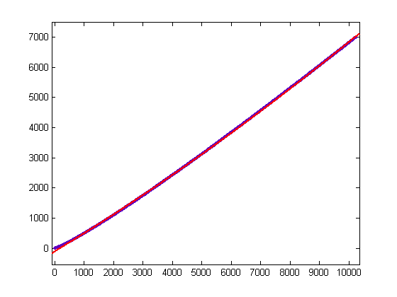
For a quadratic least-squares fit of Σi=1x(n[x/i]-m[x/i])d(i) versus x for x=2, 3, 4, ..., 10250, p1=1.016e-5 with a 95% confidence interval of (1.011e-5, 1.021e-5), p2=0.5924 with a 95% confidence interval of (0.5918, 0.5929), p3=-106.6 with a 95% confidence interval of (-107.8, -105.4), SSE=4.373e+6, R-square=0.9999, and RMSE=20.66. A plot of log(x!)/12-Σi=1x(n[x/i]-m[x/i])d(i) versus x for x=2, 3, 4, ..., 40000 is;
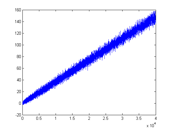
A plot of 5Σi=1x(m[x/i]-n[x/i]+1/6 )σ0(i) versus x for x=2, 3, 4, ..., 5000 is;

For a linear least-squares fit of 5Σi=1x(m[x/i]-n[x/i]+1/6)σ0(i) versus x for x=2, 3, 4, ..., 5000, p1=0.999 with a 95% confidence interval of (0.9985, 0.9994), p2=0.003815 with a 95% confidence interval of (-1.233, 1.24), SSE=2.481e+6, R-square=0.9998, and RMSE=22.28. For a linear least-squares fit of 5Σi=1x(m[x/i]-n[x/i]+1/6)σ0(i) versus x for x=2, 3, 4, ..., 40000, p1=0.9989 with a 95% confidence interval of (0.9989, 0.9989), p2=0.136 with a 95% confidence interval of (-0.6118, 0.88381), SSE=5.821e+7, R-square=1, and RMSE=38.15.
Σi=1xM([x/i])σ1(i)=x(x+1)/2. A plot of x(x+1)/24 and Σi=1x(n[x/i]-m[x/i])σ1(i) versus x for x=2, 3, 4, ..., 10250 is;
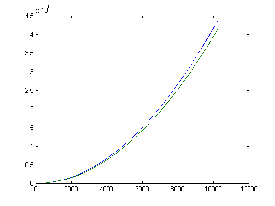
For a quadratic least-squares fit of Σi=1x(n[x/i]-m[x/i])σ1(i) versus x for x=2, 3, 4, ..., 10250, p1=0.03945 with a 95% confidence interval of (0.03945, 0.03946), p2=-0.04567 with a 95% confidence interval of (-0.06933, -0.02201), p3=2.278 with a 95% confidence interval of (-50.24, 54.8), SSE=8.366e+9, R-square=1, and RMSE=903.6. For a quadratic least-squares fit of Σi=1x(n[x/i]-m[x/i])σ1(i) versus x for x=2, 3, 4, ..., 40000, p1=0.03945 with a 95% confidence interval of (0.03945, 0.03945), p2=-0.04398 with a 95% confidence interval of (-0.05599, -0.03197), p3=0.4941 with a 95% confidence interval of (-103.5, 104.5), SSE=5.004e+11, R-square=1, and RMSE=3537. A plot of x(x+1)/2 and 5.13Σi=1x(m[x/i]-n[x/i]+1/6)σ1(i) versus x for x=2, 3, 4, ..., 100 is;
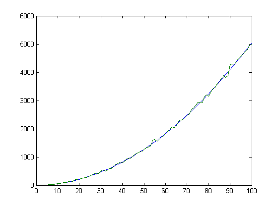
Σi=1xM([x/i])σ2(i)=x(x+1)(2x+1)/6. A plot of x(x+1)(2x+1)/6 and 5.36Σi=1x(m[x/i]-n[x/i]+1/6)σ2(i) versus x for x=2, 3, 4, ..., 200 is;
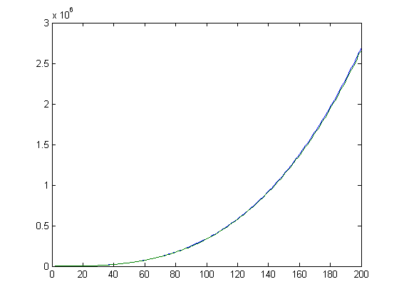
Ramanujan proved that the Riemann hypothesis implies σ1(n)<eγnlog(log(n)) for sufficiently large n where γ denotes Euler's constant. (Robin proved that this inequality is true for all n≥5041 if and only if the Riemann hypothesis is true.) A plot of M(x)+eγΣi=2xM([x/i])ilog(log(i)), 12((nx-mx)+eγΣi=2x(n[x/i]-m[x/i])ilog(log(i))), and x(x+1)/2 versus x for x=2, 3, 4, ..., 200 is;
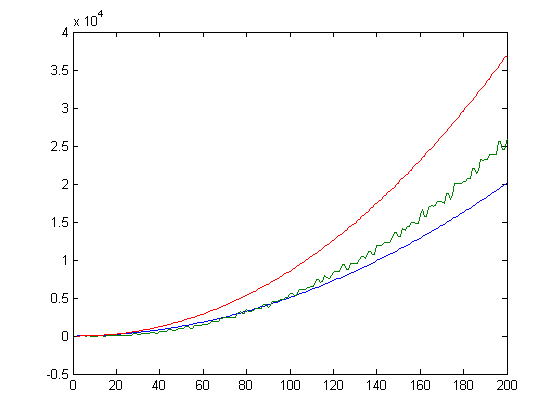
A plot of M(x)+eγΣi=2xM([x/i])ilog(log(i))-5.14((mx-nx+1/6)+eγΣi=2x(m[x/i]-n[x/i]+1/6)ilog(log(i))) versus x for x=2, 3, 4, ..., 1000 is;
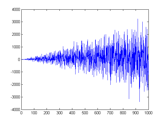
A plot of M(x)+eγΣi=2xM([x/i])ilog(log(i)), eγA(x), and x(x+1)/2 versus x for x=2, 3, 4, ..., 200 is;
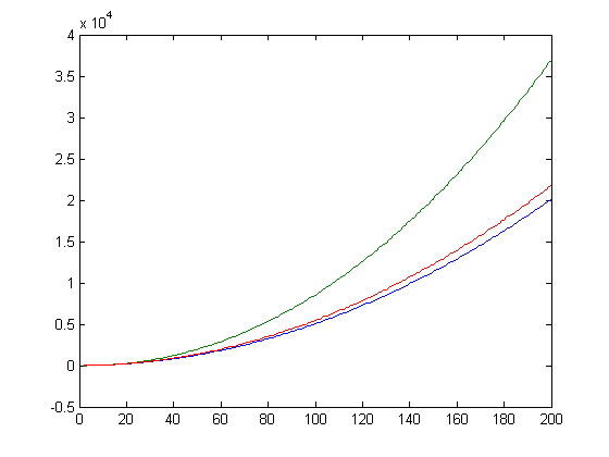
eγA(x)>x(x+1)/2, eγΣi=1xsgn(M([x/i]))i>Σi=1xsgn(M([x/i]))σ1(i), and eγΣi=1x|sgn(M([x/i]))|i>Σi=1x|sgn(M([x/i]))|σ1(i). (These inequalities are related to Bachmann's theorem that σ(1)+σ(2)+...+σ(n)=(1/12)π2n2+O(nlog n)). A plot of |M(x)|+eγΣi=2x|M([x/i])|ilog(log(i)), Σi=1x|M([x/i])|σ1(i), 12(|nx-mx|+eγΣi=2x|n[x/i]-m[x/i]|ilog(log(i))), and A(x) versus x for x=2, 3, 4, ..., 200 is;
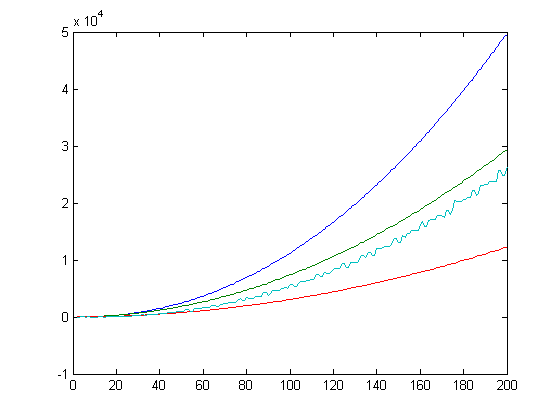
A plot of sgn(M(x))+eγΣi=2xsgn(M([x/i]))ilog(log(i)), 12(sgn(nx-mx)+eγΣi=2xsgn(n[x/i]-m[x/i])ilog(log(i))), and Σi=1xsgn(M([x/i]))σ1(i), versus x for x=2, 3, 4, ..., 200 is;
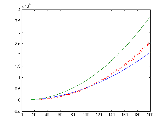
2+eγA(x)>Σi=1xsgn(M([x/i]))σ1(i). (Upper bounds of partial sums of Σi=1xsgn(M([x/i]))σ1(i) are determined in the following.) A plot of M(x)+eγΣi=2xM([x/i])ilog(log(i)), 12((nx-mx)+eγΣi=2x(n[x/i]-m[x/i])ilog(log(i))), and x(x+1)/2 versus x for x=2, 3, 4, ..., 10250 is;
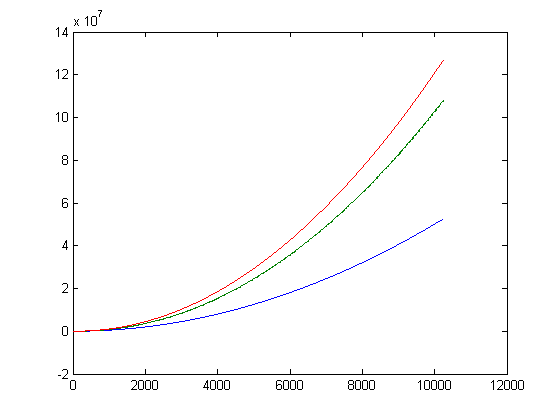
For a quadratic least-squares fit of M(x)+eγΣi=2xM([x/i])ilog(log(i)) versus x for x=2, 3, 4, ..., 10250, p1=1.253 with a 95% confidence interval of (1.253, 1.253), p2=-485.3 with a 95% confidence interval of (-487.5, -483.1), p3=2.93e+5 with a 95% confidence interval of (2.881e+5, 2.979e+5), SSE=7.322e+13, R-square=1, and RMSE=8.453e+4. For a quadratic least-squares fit of 12((nx-mx)+eγΣi=2x(n[x/i]-m[x/i])ilog(log(i))) versus x for x=2, 3, 4, ..., 10250, p1=1.081 with a 95% confidence interval of (1.081, 1.081), p2=-587.5 with a 95% confidence interval of (-590.2, -584.8), p3=3.46e+5 with a 95% confidence interval of (3.401e+5, 3.519e+5), SSE=1.061e+14, R-square=1, and RMSE=1.018e+5. Let Hn=Σj=1n1/j. Lagarias proved that Σd|nd≤Hn+exp(Hn)log(Hn) (with equality only for n=1) if and only if the Riemann hypothesis is true. A plot of Σi=1xM([x/i])(Hn+exp(Hn)log(Hn)), 12Σi=1x(n[x/i]-m[x/i])(Hn+exp(Hn)log(Hn)), and x(x+1)/2 versus x=2, 3, 4, ..., 200 is;
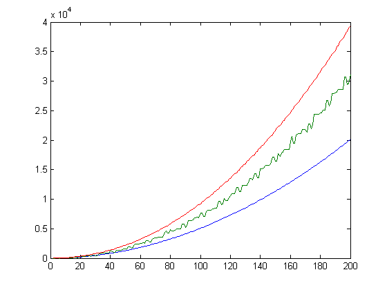
A plot of Σi=1xM([x/i])(Hn+exp(Hn)log(Hn)) and 5.134Σi=1x(m[x/i]-n[x/i]+1/6)(Hn+exp(Hn)log(Hn)) (superimposed on each other) versus x for x=2, 3, 4, ..., 5000 is;
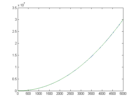
A plot of Σi=1xM([x/i])(Hn+exp(Hn)log(Hn))-5.134Σi=1x(m[x/i]-n[x/i]+1/6)(Hn+exp(Hn)log(Hn)) versus x for x=2, 3, 4, ..., 5000 is;
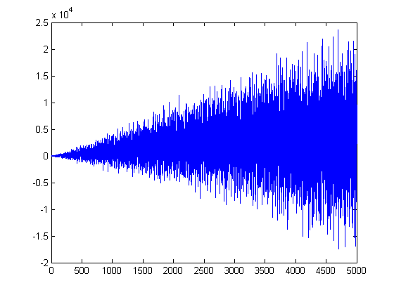
A plot of Σi=1xd(i)-xlog(x)/2 versus x for x=2, 3, 4, ..., 3000 is;
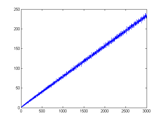
A plot of log(x!), Σi=1xlog(i)/d(i), and Σi=1xM([x/i])2 versus x for x=2, 3, 4, ..., 2000 is;
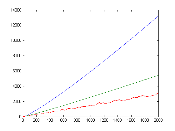
A plot of ψ(x) and Σi=1x(n[x/i]-m[x/i])log(i) versus x for x=2, 3, 4, ..., 10250 is;
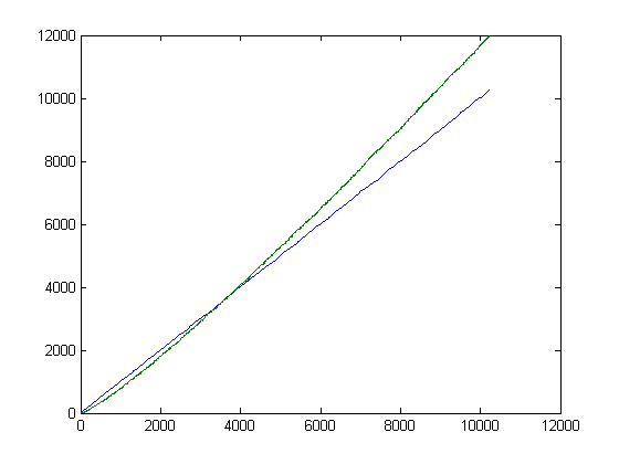
ψ(x) is the more linear of the two curves. For a quadratic least-squares fit of Σi=1x(n[x/i]-m[x/i])log(i) versus x for x=2, 3, 4, ..., 10250, p1=2.006e-5 with a 95% confidence interval of (1.995e-5, 2.017e-5), p2=0.9945 with a 95% confidence interval of (0.9933, 0.9957), p3=-215.9 with a 95% confidence interval of (-218.5, -213.2), SSE=2.103e+7, R-square=0.9998, and RMSE=45.3. A plot of log(x!)-6Σi=1x(n[x/i]-m[x/i])log(i) versus x for x=2, 3, 4, ..., 40000 is;
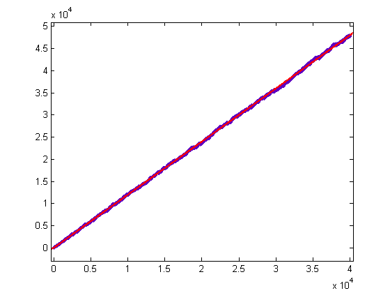
For a linear least-squares fit of log(x!)-6Σi=1x(n[x/i]-m[x/i])log(i) versus x for x=2, 3, 4, ..., 40000, p1=1.201 with a 95% confidence interval of (1.201, 1.201), p2=-31.92 with a 95% confidence interval of (-35.4, -28.44), SSE=1.262e+9, R-square=0.9998, and RMSE=177.6. A plot of 5Σi=1x(m[x/i]-n[x/i]+1/6)log(i) versus x for x=2, 3, 4, ..., 5000 is;
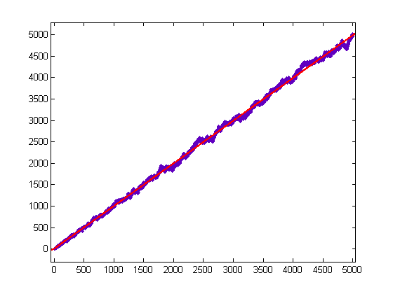
For a linear least-squares fit of 5Σi=1x(m[x/i]-n[x/i]+1/6)log(i) versus x for x=2, 3, 4, ..., 5000, p1=0.9959 with a 95% confidence interval of (0.9949, 0.997), p2=4.395 with a 95% confidence interval of (1.411, 7.379), SSE=1.445e+7, R-square=0.9986, and RMSE=53.78. For a linear least-squares fit of 5Σi=1x(m[x/i]-n[x/i]+1/6)log(i) versus x for x=2, 3, 4, ..., 40000, p1=1.001 with a 95% confidence interval of (1.001, 1.001), p2=-26.6 with a 95% confidence interval of (-29.5, -23.7), SSE=8.765e+8, R-square=0.9998, and RMSE=148.
A plot of log(x!) and Σi=1x(n[x/i]-m[x/i])log(i)d(i) versus x for x=2, 3, 4, ..., 10250 is;
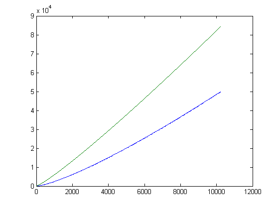
A plot of log(x!)-Σi=1x(n[x/i]-m[x/i])log(i)d(i) versus x for x=2, 3, 4, ..., 10250 is;
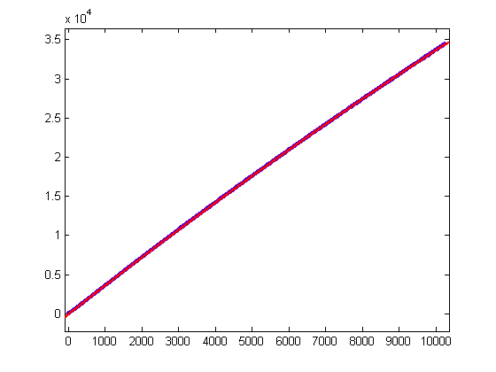
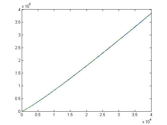
For a quadratic least-squares fit of log(x!)-Σi=1x(n[x/i]-m[x/i])log(i)d(i) versus x for x=2, 3, 4, ..., 10250, p1=-3.112e-5 with a 95% confidence interval of (-3.118e-5, -3.106e-5), p2=3.684 with a 95% confidence interval of (3.684, 3.685), p3=-97.64 with a 95% confidence interval of (-99.09, -96.19), SSE=6.402e+6, R-square=1, and RMSE=25. For a quadratic least-squares fit of log(x!)-Σi=1x(n[x/i]-m[x/i])log(i)d(i) versus x for x=2, 3, 4, ..., 40000, p1=-1.506e-5 with a 95% confidence interval of (-1.508e-5, -1.504e-5), p2=3.409 with a 95% confidence interval of (3.409, 3.41), p3=746.4 with a 95% confidence interval of (738.8, 753.9), SSE=2.655e+9, R-square=0.9999, and RMSE=257.6. A plot of 5Σi=1x(m[x/i]-n[x/i]+1/6)log(i)d(i) and log(x!) (superimposed on each other) versus x for x=2, 3, 4, ..., 40000 is;
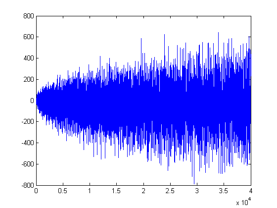
A plot of log(x!)-4.99Σi=1x(m[x/i]-n[x/i]+1/6)log(i)d(i) versus x for x=2, 3, 4, ..., 40000 is;
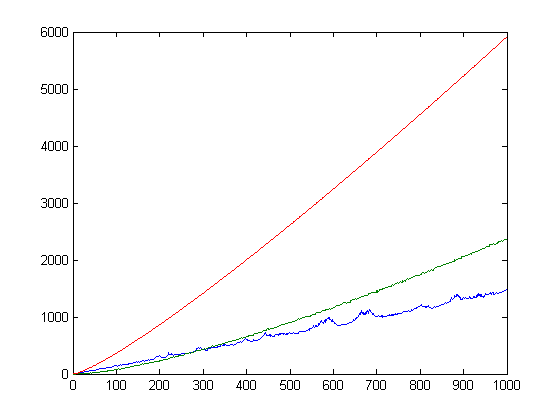
A plot of log(x!), Σi=1x(n[x/i]-m[x/i])log(i)d(i), and Σi=1xM([x/i])2 versus x for x=2, 3, 4, ..., 1000 is;
Also, 2/3≥(1/x)Σi=1x|sgn(M([x/i]))|-(1/x)Σi=1xsgn(M([x/i])). Also, Σi=1xsgn(M([x/i])) is approximately equal to Σi=1x|sgn(n[x/i]-m[x/i])| (for x≤5128, 16≥|Σi=1xsgn(M([x/i]))-Σi=1x|sgn(n[x/i]-m[x/i])|) and Σi=1x|sgn(n[x/i]-m[x/i])|≥Σi=1xsgn(n[x/i]-m[x/i]). A plot of Σi=1xsgn(M([x/i])) and Σi=1x|sgn(n[x/i]-m[x/i])|-20 versus x for x=2, 3, 4, ..., 5128 is;
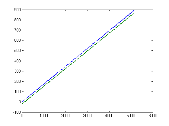
For a linear least-squares fit of Σi=1xsgn(M([x/i])) versus x for x=2, 3, 4, ..., 10250, p1=0.1739 with a 95% confidence interval of (0.1739, 0.1739), p2=0.1087 with a 95% confidence interval of (0.004574, 0.2128), SSE=7.402e+4, R-square=1, and RMSE=2.688. For a linear least-squares fit of Σi=1x|sgn(n[x/i]-m[x/i])| versus x for x=2, 3, 4, ..., 10250, p1=0.1727 with a 95% confidence interval of (0.1727, 0.1727), p2=-0.4368 with a 95% confidence interval of (-0.5234, -0.3502), SSE=5.122e+4, R-square=1, and RMSE=2.236. A plot of √Σi=1xsgn(M([x/i]))-√Σi=1x|sgn(n[x/i]-m[x/i])| versus x for x=2, 3, 4, ..., 5128 is;
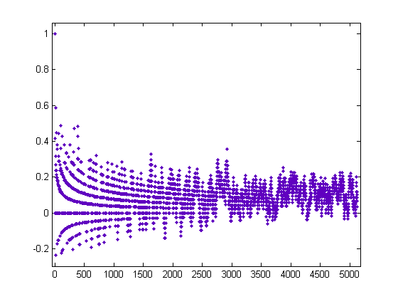
A plot of (1/x)Σi=1xsgn(M([x/i]))-(1/x)Σi=1x|sgn(n[x/i]-m[x/i])| versus x for x=2, 3, 4, ..., 170 is;
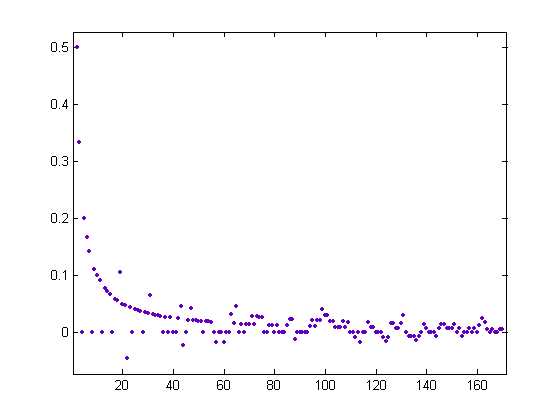
The arc beginning with the value 0.5 consists of terms from the harmonic sequence. Another arc consists of the terms -1/22, -1/44, -1/57, -1/60, -1/88, -1/112, -1/123, -1/125, -1/133, -1/134, -1/135, -1/137, -1/144, -1/153, .... Another arc consists of the terms -2/114, -2/124, -2/136, .... Another arc consists of the terms 2/19, 2/31, 2/43, 2/47, 2/63, 2/73, 2/74, 2/75, 2/86, 2/87, 2/95, 2/97, 2/98, 2/102, 2/103, 2/107, 2/109, 2/117, 2/126, 2/127, 2/130, 2/139, 2/146, 2/147, 2/151, 2/161, ... Another arc consists of the terms 3/65, 3/100, 3/101, 3/163, .... Another arc consists of the terms 4/99, 4/131, 4/162, .... For x in the vicinity of 10250, (1/x)Σi=1xsgn(M([x/i]))-(1/x)Σi=1x|sgn(n[x/i]-m[x/i])| is less than 0.0025.
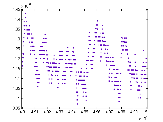
A plot of (1/x)Σi=1xsgn(M([x/i]))-(1/x)Σi=1x|sgn(n[x/i]-m[x/i])| versus x for x=49000, 49001, 49002,..., 50000 is;
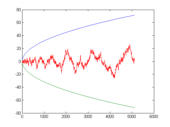
If x>56, g(x)>12Σi=1x(n[x/i]-m[x/i])i and if x>78, (h(x))2>Σi=1x(n[x/i]-m[x/i])i. Also, Σi=1x(n[x/i]-m[x/i])i≥Σi=1xsgn(n[x/i]-m[x/i])i. In general, mx-nx corresponds to M(x). A "Riemann hypothesis" for the Farey sequence is that nx-mx=O(x½).
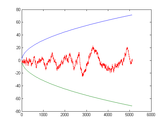
The following two plots show the correspondence between mx-nx and M(x). A plot of M(x) for x=2, 3, 4, ..., 5128 is;
A plot of mx-nx for x=2, 3, 4, ..., 5128 is;
Constraints on the growth of |mx-nx| are determined by the density of the primes. In the following, lower and upper bounds of mx (and nx) are determined. Denote the lower bound by L(x) and the upper bound by U(x). U(x)-L(x)=3+Σ[logq(x)]+Σ[logq(x/2)] where the summation is over the primes q of the form 4k+3 that are less than or equal to x. A plot of 1.5x/log(x)-(U(x)-L(x)) versus x for x=2, 3, 4, ..., 50000 is;
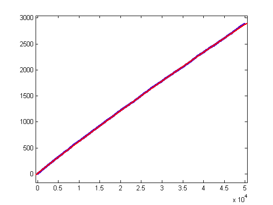
For a quadratic least-squares fit of 1.5x/log(x)-(U(x)-L(x)) versus x for x=2, 3, 4, ..., 50000, p1=-9.077e-8 with a 95% confidence interval of (-9.104e-8, -9.05e-8), p2=0.06182 with a 95% confidence interval of (0.06181, 0.06184), p3=10.07 with a 95% confidence interval of (9.92, 10.23), SSE=1.689e+6, R-square=1, and RMSE=5.812. For a quadratic least-squares fit of 1.5x/log(x)-(U(x)-L(x)) versus x for x=2, 3, 4, ..., 100000, p1=-4.287e-8 with a 95% confidence interval of (-4.295e-8, -4.279e-8), p2=0.05926 with a 95% confidence interval of (0.05925, 0.05927), p3=32.53 with a 95% confidence interval of (32.34, 32.71), SSE=9.426e+6, R-square=1, and RMSE=9.709. A plot of 1.5x/log(x) and U(x)-L(x) versus x for x=2, 3, 4, ..., 200 is;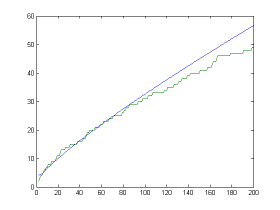
A plot of √(U(x)-L(x)) and |nx-mx| versus x for x=2, 3, 4, ..., 50000 is;
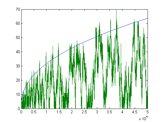
A histogram of the mx-nx values for x=2, 3, 4, ..., 10000 superimposed on a normal probability distribution having the same mean and standard deviation (-0.9805 and 12.6148 respectively) is;
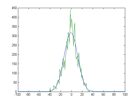
Let s(x) denote the standard deviation of the distribution of mi-ni values from i=2 to x. A plot of 3+2.4s(x) and √(U(x)-L(x)) versus x for x=2, 3, 4, ..., 20000 is;
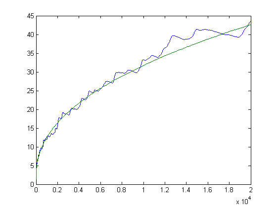
A plot of s(x) and 0.385√(x/log(x)) versus x for x=2, 3, 4, ..., 50000 is;
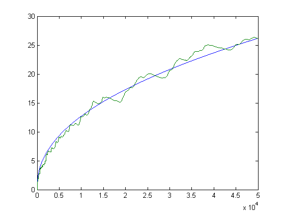
Let ox denote the number of fractions less than 1/5 and px the number of fractions greater than 1/5 and less than 2/5 in a Farey sequence of order x. A plot of upper and lower bounds of ox (computed by determining whether 5 divides φ(n)) and ox for x=2, 3, 4, ..., 200 is;
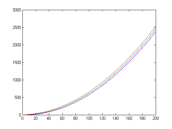
A plot of the square root of the corresponding upper bound minus the corresponding lower bound and |ox-px| for x=2, 3, 4, ..., 12000 is;
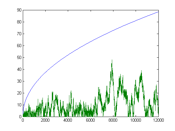
Let qx denote the number of fractions less than 1/6 and rx the number of fractions greater than 1/6 and less than 1/3 in a Farey sequence of order x. A plot of the square root of the corresponding upper bound minus the corresponding lower bound and |qx-rx| for x=2, 3, 4, ..., 12000 is;
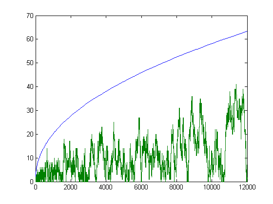
Let s(x) denote the standard deviation of the distribution of qi-ri values from i=2 to x. A plot of 5.2s(x) and the square roots of the upper bounds minus the lower bounds for x=2, 3, 4, ..., 10000 is;
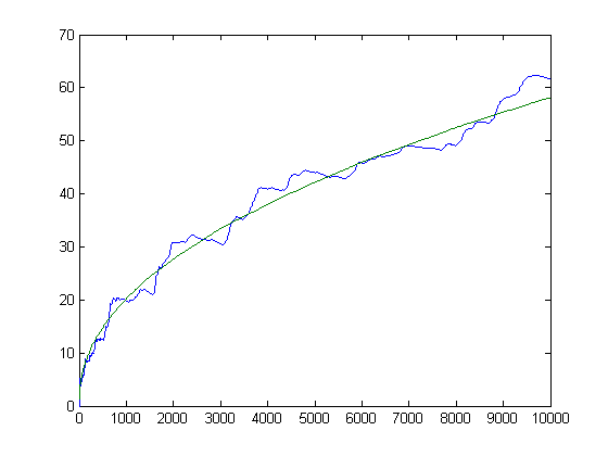
Let sx denote the number of fractions less than 1/7 and tx the number of fractions greater than 1/7 and less than 2/7 in a Farey sequence of order x. A plot of the square root of the corresponding upper bound minus the corresponding lower bound and |sx-tx| for x=2, 3, 4, ..., 12000 is;
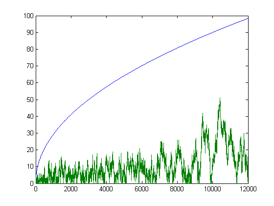
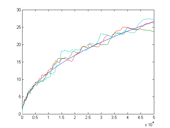
Let ux denote the number of fractions less than 1/8 and vx the number of fractions greater than 1/8 and less than 1/4 in a Farey sequence of order x. A plot of the standard deviations of the distributions of mi-ni, qi-ri, and ui-vi values from i=2 to x and (1/8.4)√x versus x for x=2, 3, 4, ..., 50000 is;
Let h5(x) denote Σi=1x(p[x/i]-o[x/i]), let h6(x) denote Σi=1x(r[x/i]-q[x/i]), let h7(x) denote Σi=1x(t[x/i]-s[x/i]), and let h8(x) denote Σi=1x(v[x/i]-u[x/i]). Based on empirical evidence, h5(x+5)=h5(x)+2, h6(x+6)=h6(x)+2, h7(x+7)=h7(x)+3, and h8(x+8)=h8(x)+3. (p3 and p4 are set to 1 and 2 respectively, r4 and r5 are set to 1 and 2 respectively, t4, t5, and t6 are set to 1, 2, and 3 respectively, and v5, v6, and v7 are set to 1, 2, and 3 respectively. If n3 is set to 1 instead of 0, then h(x+4)=h(x)+1.) These slopes determine the factors required to "linearize" Σi=1x(p[x/i]-o[x/i])log(i), Σi=1x(r[x/i]-q[x/i])log(i), Σi=1x(t[x/i]-s[x/i])log(i), and Σi=1x(v[x/i]-u[x/i])log(i). As previously shown, the factor required for Σi=1x(n[x/i]-m[x/i])log(i) is 12/2. A plot of log(x!)-(5/2)Σi=1x(p[x/i]-o[x/i])log(i) versus x for x=2, 3, 4, ..., 10000 is;
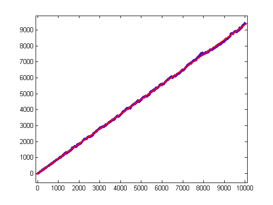
A plot of log(x!)-(6/2)Σi=1x(r[x/i]-q[x/i])log(i) versus x for x=2, 3, 4, ..., 10000 is;
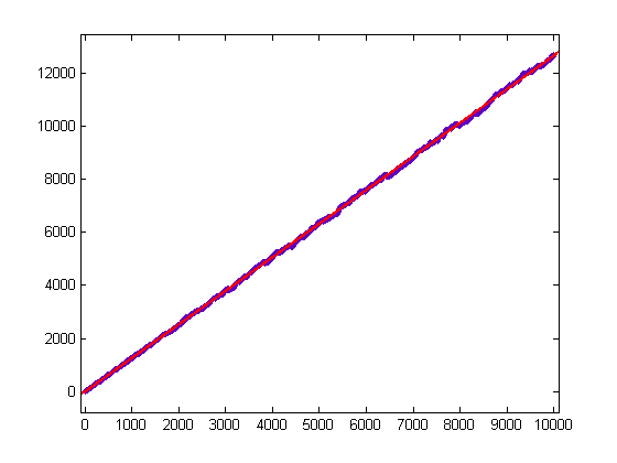
A plot of log(x!)-(7/3)Σi=1x(t[x/i]-s[x/i])log(i) versus x for x=2, 3, 4, ..., 10000 is;
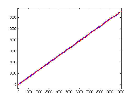
A plot of (2/5)log(x!)-Σi=1x(p[x/i]-o[x/i])σ0(i) versus x for x=2, 3, 4, ..., 10000 is;
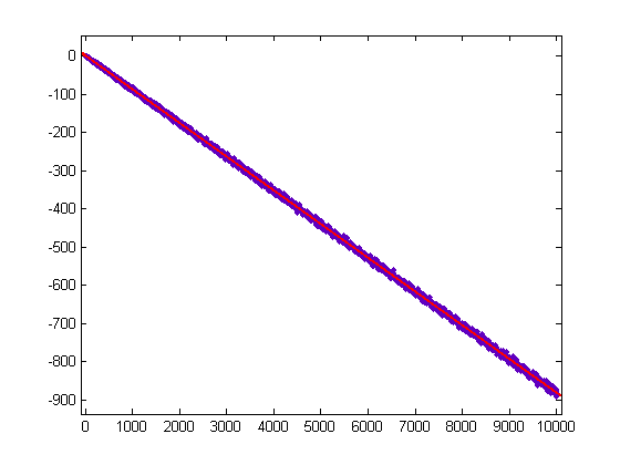
A plot of (2/6)log(x!)-Σi=1x(r[x/i]-q[x/i])σ0(i) versus x for x=2, 3, 4, ..., 10000 is;

A plot of (3/7)log(x!)-Σi=1x(t[x/i]-s[x/i])σ0(i) versus x for x=2, 3, 4, ..., 10000 is;
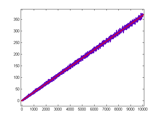
For a quadratic least-squares fit of log(x!)-(2/5)Σi=1x(p[x/i]-o[x/i])log(i)d(i) versus x for x=2, 3, 4, ..., 10000, p1=-3.041e-5 with a 95% confidence interval of (-3.045e-5, -3.037e-5), p2=3.553 with a 95% confidence interval of (3.553, 3.553), p3=-93.21 with a 95% confidence interval of (-94.15, -92.27), SSE=2.549e+6, R-square=1, and RMSE=15.97. For a quadratic least-squares fit of log(x!)-(1/2)Σi=1x(r[x/i]-q[x/i])log(i)d(i) versus x for x=2, 3, 4, ..., 10000, p1=-2.999e-5 with a 95% confidence interval of (-3.003e-5, -2.995e-5), p2=3.763 with a 95% confidence interval of (3.762, 3.763), p3=-113.8 with a 95% confidence interval of (-114.7, -112.9), SSE=2.437e+6, R-square=1, and RMSE=15.61. For a quadratic least-squares fit of log(x!)-(3/7)Σi=1x(t[x/i]-s[x/i])log(i)d(i) versus x for x=2, 3, 4, ..., 10000, p1=-4.499e-5 with a 95% confidence interval of (-4.507e-5, -4.491e-5), p2=3.464 with a 95% confidence interval of (3.463, 3.465), p3=-6.292 with a 95% confidence interval of (-8.189, -4.394), SSE=1.039e+7, R-square=1, and RMSE=32.25.
A plot of log(x!)-2.3679Σi=1x(q[x/i]-r[x/i]+1/3)log(i)d(i) versus x for x=2, 3, 4, ..., 40000 is;
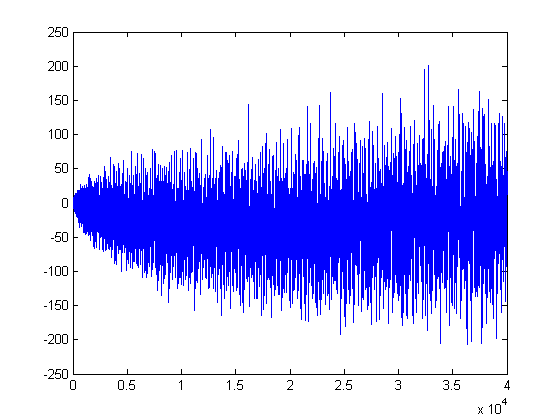
For a linear least-squares fit of 2.3725Σi=1x(q[x/i]-r[x/i]+1/3)σ0(i) versus x for x=2, 3, 4, ..., 40000, p1=1 with a 95% confidence interval of (1, 1), p2=0.1345 with a 95% confidence interval of (-0.08722, 0.3563), SSE=5.118e+6, R-square=1, and RMSE=11.31. For a linear least-squares fit of 2.3730Σi=1x(q[x/i]-r[x/i]+1/3)log(i) versus x for x=2, 3, 4, ..., 40000, p1=1 with a 95% confidence interval of (0.9999, 1), p2=2.909 with a 95% confidence interval of (1.367, 4.451), SSE=2.476e+8, R-square=1, and RMSE=78.67.
A plot of log(x!)-1.793Σi=1x(s[x/i]-t[x/i]+3/7)log(i)d(i) versus x for x=2, 3, 4, ..., 40000 is;
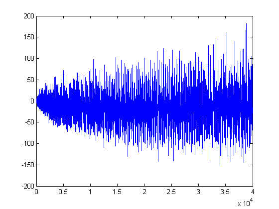
For a linear least-squares fit of 1.795Σi=1x(s[x/i]-t[x/i]+3/7)σ0(i) versus x for x=2, 3, 4, ..., 40000, p1=1 with a 95% confidence interval of (1, 1), p2=0.1419 with a 95% confidence interval of (-0.04282, 0.3266), SSE=3.551e+6, R-square=1, and RMSE=9.422. For a linear least-squares fit of 1.794Σi=1x(s[x/i]-t[x/i]+3/7)log(i) versus x for x=2, 3, 4, ..., 40000, p1=0.9999 with a 95% confidence interval of (0.9999, 0.9999), p2=-6.001 with a 95% confidence interval of (-7.125, -4.878), SSE=1.313e+8, R-square=1, and RMSE=57.3.
Let yx(n) denote the number of fractions less than 1/n and zx(n) the number of fractions greater than 1/n and less than 2/n in a Farey sequence of order x. A plot of the p1 values of the linear least-squares fits of Σi=1x(y[x/i](n)-z[x/i](n)+[(n-1)/2]/n)σ0(i) versus x for x=2, 3, 4, ..., 4000 and n=4, 5, 6, ..., 15 is;
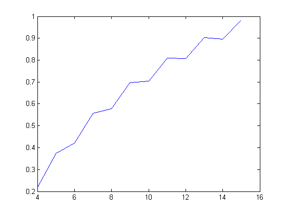
A quadratic least-squares fit of the p1 values of the linear least-squares fits of Σi=1x(y[x/i](n)-z[x/i](n)+[(n-1)/2]/n)σ0(i) versus x for x=2, 3, 4, ..., 4000 and n=4, 6, 8, ..., 14 is;
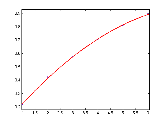
A quadratic least-squares fit of the p1 values of the linear least-squares fits of Σi=1x(y[x/i](n)-z[x/i](n)+[(n-1)/2]/n)σ0(i) versus x for x=2, 3, 4, ..., 4000 and n=5, 7, 9, ..., 15 is;

A plot of the p1 and p2 values of the quadratic least-squares fits of Σi=1x(y[x/i](n)-z[x/i](n)+[(n-1)/2]/n)σ1(i) versus x for x=2, 3, 4, ..., 4000 and n=4, 5, 6, ..., 15 is;
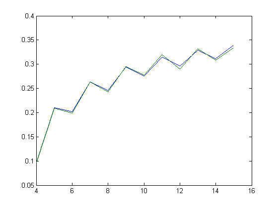
A quartic least-squares fit of the p1 values of the quadratic least-squares fits of Σi=1x(y[x/i](n)-z[x/i](n)+[(n-1)/2]/n)σ1(i) versus x for x=2, 3, 4, ..., 4000 and n=4, 6, 8, ..., 14 is;
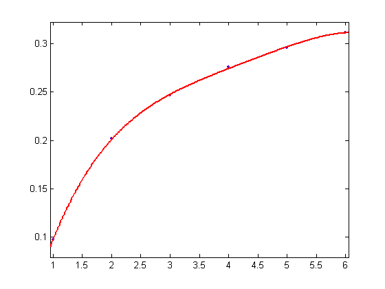
A quartic least-squares fit of the p1 values of the quadratic least-squares fits of Σi=1x(y[x/i](n)-z[x/i](n)+[(n-1)/2]/n)σ1(i) versus x for x=2, 3, 4, ..., 4000 and n=5, 7, 9, ..., 15 is;
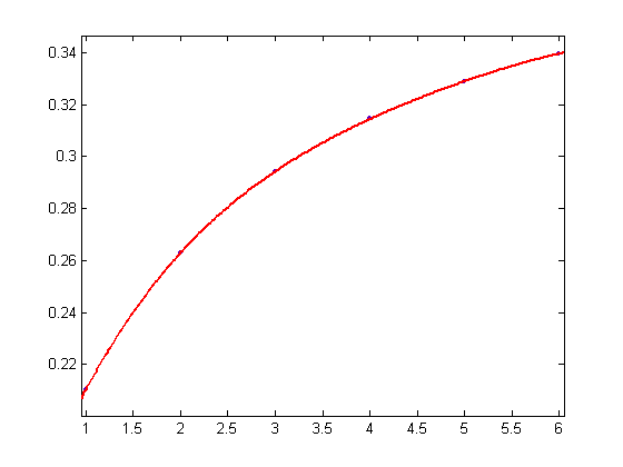
A sixth-order polynomial least-squares fit of the p1 values of the cubic least-squares fits of Σi=1x(y[x/i](n)-z[x/i](n)+[(n-1)/2]/n)σ2(i) versus x for x=2, 3, 4, ..., 2000 and n=5, 7, 9, ..., 31 is;
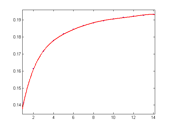
A plot of yx(65)-zx(65) versus x for x=2, 3, 4, ..., 1625 is;
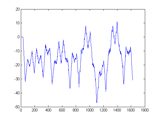
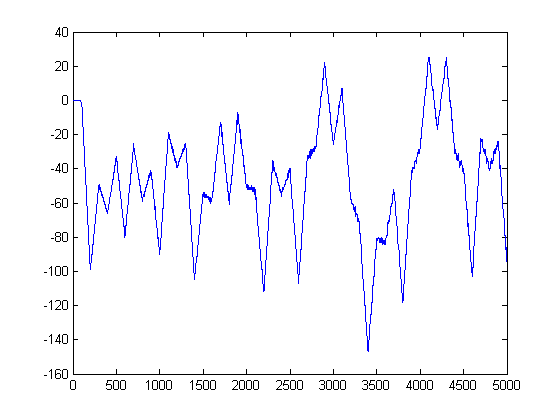
A plot of yx(200)-zx(200) versus x for x=2, 3, 4, ..., 5000 is;
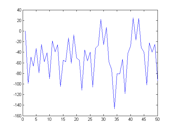
A plot of yx(200)-zx(200) versus x for x=100, 200, 300, 400, ..., 5000 is;
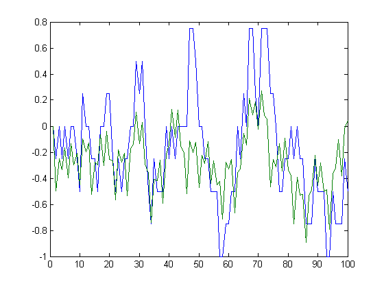
For even n, the limits of (yn/2(n)-zn/2(n))/n, (yn(n)-zn(n))/n, (y3n/2(n)-z3n/2(n))/n, (y2n(n)-z2n(n))/n,..., as n approaches infinity appear to be -1/2, -1/4, -1/3, -1/6, -2/5, -2/15, -31/105, -29/140, -19/42, -41/420, -76/385, -201/1540, -751/1430, -1109/4004, -803/2718, -857/13411, -3577/11807, -721/17163, -738/2897, ..., respectively. Superimposed plots of (y2(4)-z2(4))/4, (y4(4)-z4(4))/4, (y6(4)-z6(4))/4, ..., (y200(4)-z200(4))/4 and (y500000(1000000)-z500000(1000000))/1000000, (y1000000(1000000)-z1000000(1000000))/1000000, (y1500000(1000000)-z1500000(1000000))/1000000, ..., (y50000000(1000000)-z50000000(1000000))/1000000 are;
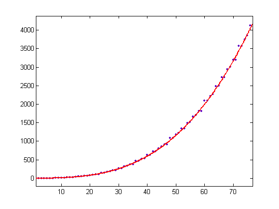
Let δm(x), m=1, 2, 3, ..., denote the interpolated normalized difference in the number of fractions in a Farey sequence computed using the above limits (m-1 values between successive limits are interpolated). A cubic least-squares fit of -Σi=1xδ4([x/i])σ2(i) versus x for x=2, 3, 4, ..., 76 is;
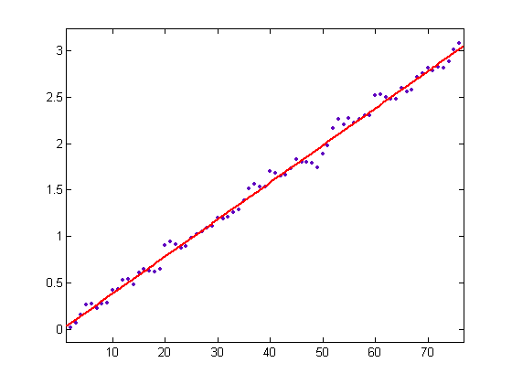
These values were computed using 19 limits. A quadratic least-squares fit of -Σi=1xδ4([x/i])σ1(i) versus x for x=2, 3, 4, ..., 76 is;
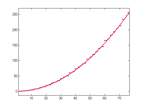
A linear least-squares fit of Σi=1xδ4([x/i])2 versus x for x=2, 3, 4, ..., 76 is;
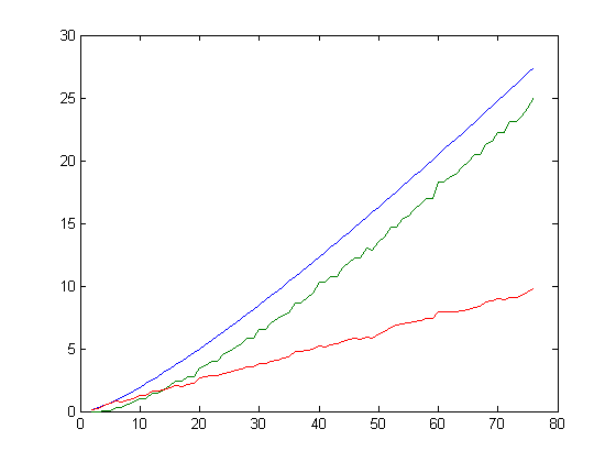
A plot of (1/12)xlog(x), -Σi=1xδ4([x/i])log(i), and -Σi=1xδ4([x/i]) versus x for x=2, 3, 4, ... 76 is;
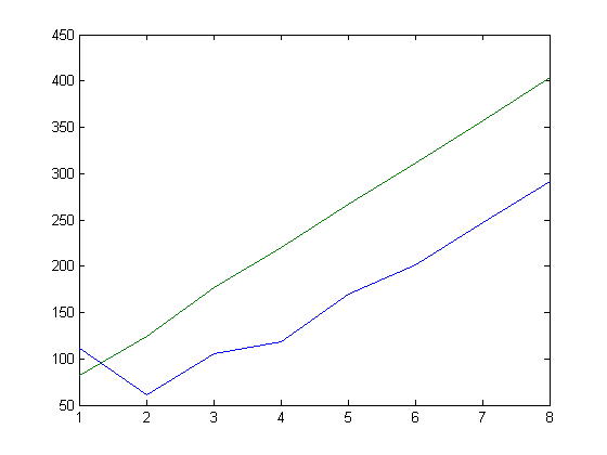
When a small number of limits is considered, there appears to be less "noise" in the curve of Σi=1xδ1([x/i])2 values than in the curve of Σi=1xδ1([x/i]) values. A superimposed plot of the SSE values of the linear least-squares fits of Σi=1xδ1([x/i]), Σi=1xδ2([x/i]), Σi=1xδ3([x/i]), ..., Σi=1xδ8([x/i]) for x=400, 800, 1200, ..., 3200 respectively and the SSE values of the linear least-squares fits of Σi=1xδ1([x/i])2, Σi=1xδ2([x/i])2, Σi=1xδ3([x/i])2, ..., Σi=1xδ8([x/i])2 for x=400, 800, 1200, ..., 3200 respectively is;
These values were computed using 400 approximate limits (accurate to about 6 decimal places). A superimposed plot of the RMSE values of the linear least-squares fits of Σi=1xδ1([x/i]), Σi=1xδ2([x/i]), Σi=1xδ3([x/i]), ..., Σi=1xδ8([x/i]) for x=400, 800, 1200, ..., 3200 respectively and the RMSE values of the linear least-squares fits of Σi=1xδ1([x/i])2, Σi=1xδ2([x/i])2, Σi=1xδ3([x/i])2, ..., Σi=1xδ8([x/i])2 for x=400, 800, 1200, ..., 3200 respectively is;
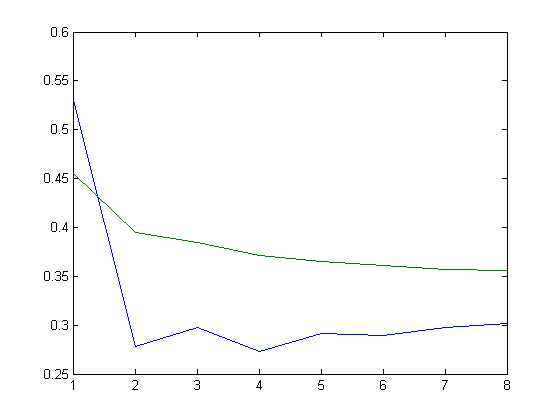
A plot of 6.6666Σi=1x(δ1([x/i])+0.1704)M(i) and Σi=1xM([x/i])M(i) versus x for x=2, 3, 4, ... 999 is;
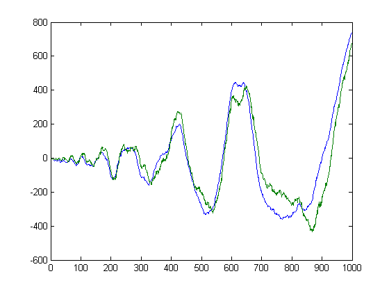
These values were computed using 1000 approximate limits. The slope of the curve of -Σi=1xδ1([x/i]) values for x=2, 3, 4, ..., 999 (as given by a linear least-squares fit) is about 0.1704.
Let L(i) denote the summatory Liouville function. A plot of √Σi=1xM([x/i])L(i)2 and √Σi=1x(δ1([x/i])+0.1704)L(i)2 versus x for x=2, 3, 4, ... 999 is;
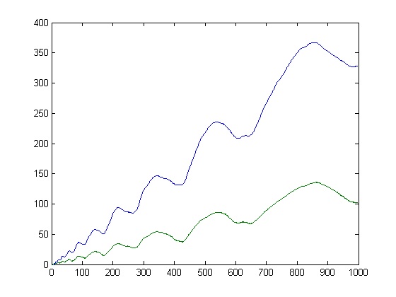
Let Λ denote the Mangoldt function. A plot of -Σi=1xδ1([x/i]) and -Σi=1xδ1([x/i])Λ(i) for x=2, 3, 4, ..., 999 is;
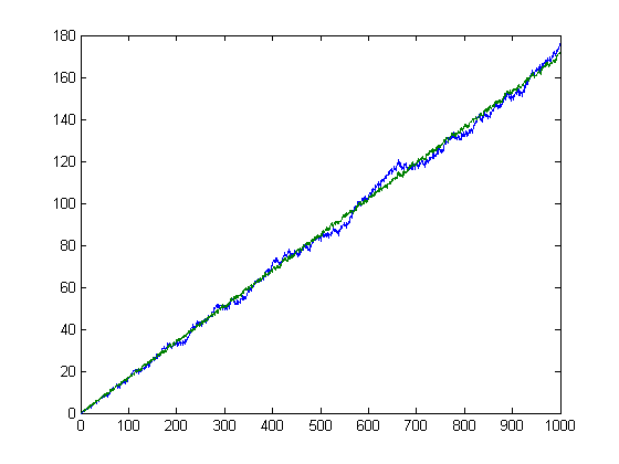
For a linear least-squares fit of -Σi=1xδ1([x/i]) versus x for x=2, 3, 4, ..., 999, p1=0.1704 with a 95% confidence interval of (0.1703, 0.1706), p2=-0.04484 with a 95% confidence interval of (-0.1291, 0.03936), SSE=455.6, R-square=0.9998, and RMSE=0.6763. For a linear least-squares fit of -Σi=1xδ1([x/i])Λ(i) versus x for x=2, 3, 4, ..., 999, p1=0.17 with a 95% confidence interval of (0.1695, 0.1705), p2=-0.2796 with a 95% confidence interval of (-0.5688, 0.009683), SSE=5374, R-square=0.9978, and RMSE=2.323. A plot of the p1 values of the linear least-squares fits of -Σi=1xδ1([x/i])Λ(i), -Σi=1xδ2([x/i])Λ(i), -Σi=1xδ3([x/i])Λ(i), ..., -Σi=1xδ36([x/i])Λ(i) versus x for x up to 999, 1999, 2999, ..., 35999 respectively is;
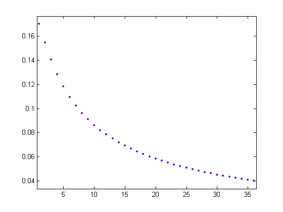
For a linear least-squares fit of -Σi=1xδ100([x/i]) versus x for x=2, 3, 4, ..., 99999, p1=0.01936 with a 95% confidence interval of (0.01936, 0.01936), p2=-0.1094 with a 95% confidence interval of (-0.1154, -0.1034), SSE=2.347e+4, R-square=1, and RMSE=0.4845. For a linear least-squares fit of -Σi=1xδ100([x/i])Λ(i) versus x for x=2, 3, 4, ..., 99999, p1=0.01936 with a 95% confidence interval of (0.01936, 0.01936), p2=-0.6391 with a 95% confidence interval of (-0.6584, -0.6198), SSE=2.415e+5, R-square=1, and RMSE=1.554. A plot of -Σi=1xδ100([x/i]) and -Σi=1xδ100([x/i])Λ(i) (superimposed on each other) for x=2, 3, 4, ..., 99999 is;
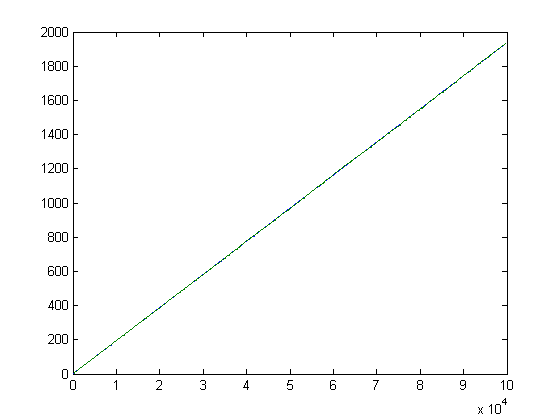
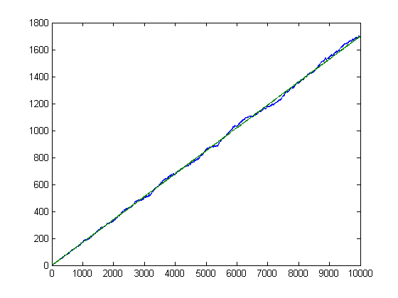
A plot of -Σi=1xδ1([x/i]) and -Σi=1xδ1([x/i])Λ(i) (where the approximate limits are accurate to about 3 decimal places) for x=2, 3, 4, ..., 9999 is;
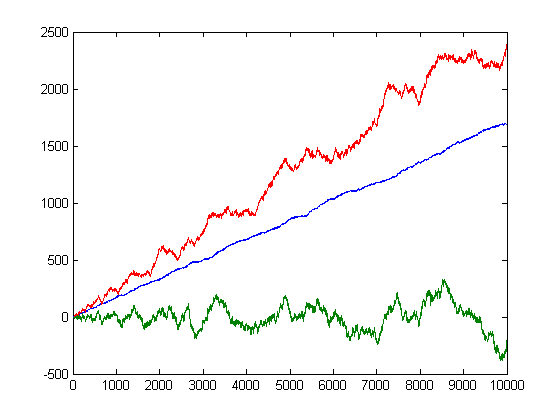
Σi=1xM([x/i])Λ(i)=-Σi=1xμ(i)log(i) where μ(i) is the Möbius function. (Σi=1xμ(i)log(i) is usually denoted by H(x). H(x)/(xlog(x))→0 as x→∞ and limx→∞(M(x)/x-H(x)/(xlog(x)))=0.) A plot of Σi=1x(z[x/i](4)-y[x/i](4))Λ(i), -Σi=1xδ1([x/i])Λ(i), and Σi=1xM([x/i])Λ(i) for x=2, 3, 4, ..., 9999 is;
Σi=1x(y[x/i](4)-z[x/i](4)+1/4)Λ(i) is approximately equal to Σi=1xM([x/i])Λ(i). A plot of (1/(xlog(x)))Σi=1x(δ1([x/i])+0.1704)Λ(i) for x=2, 3, 4, ..., 9999 is;
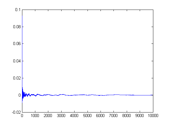
A plot of Λ*Λ (the Dirichlet product of Λ with itself) for x=2, 3, 4, ..., 999 is;
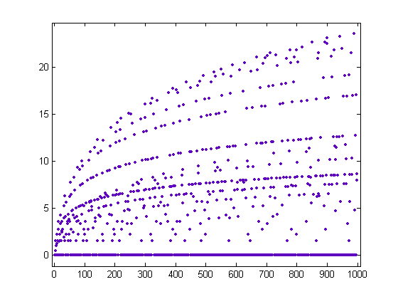
Let (α◦F)(x) denote Σn≤xα(n)F([x/n]) where α is an arithmetical function. (Usually, (α◦F)(x) denotes Σn≤xα(n)F(x/n) where F is a real or complex-valued function defined on (0, +∞) such that F(x)=0 for 0<x<1.) As expected, Λ◦(Λ◦δ1)=(Λ*Λ)◦δ1. Let u(n)=1 for all n. A quadratic least squares fit of (u◦δ1)◦δ1 (where the limits are accurate to about 6 decimal places) for x=2, 3, 4, ..., 999 is;
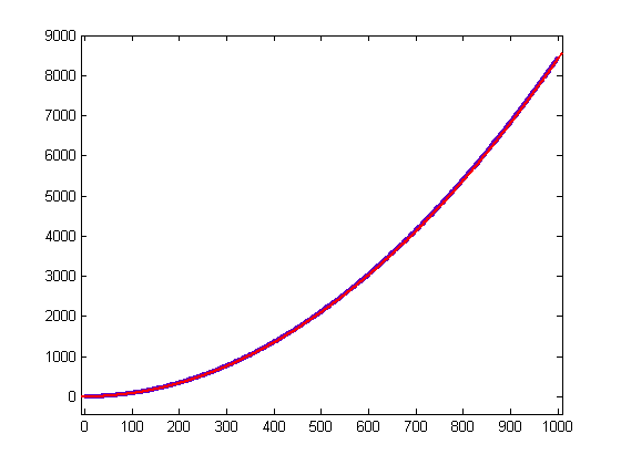
p1=0.008421 with a 95% confidence interval of (0.008414, 0.008428), p2=0.001703 with a 95% confidence interval of (-0.005279, 0.008684), p3=-0.01665 with a 95% confidence interval of (-1.53, 1.497), SSE=6.483e+4, R-square=1, and RMSE=8.072. A quadratic least-squares fit of (Λ◦δ1)◦δ1 for x=2, 3, 4, ..., 999 is;
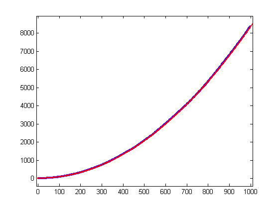
p1=0.00847 with a 95% confidence interval of (0.008459, 0.008428), p2=-0.09465 with a 95% confidence interval of (-0.1054, -0.08391), p3=4.914 with a 95% confidence interval of (2.586, 7.242), SSE=1.534e+5, R-square=1, and RMSE=12.42. For a quadratic least-squares fit of -(Λ◦δ1)◦Λ for x=2, 3, 4, ..., 999, p1=0.01802 with a 95% confidence interval of (0.01798, 0.01806), p2=-0.3354 with a 95% confidence interval of (-0.3761, -0.2946), p3=22.13 with a 95% confidence interval of (13.3, 30.97), SSE=2.208e+6 R-square=0.9999, and RMSE=47.1. Λ◦(Λ◦δ1) and δ1◦(Λ◦δ1) appear to be O(xlog(x)). A plot of -Λ◦(Λ◦δ1) for x=2, 3, 4, ..., 999 is;
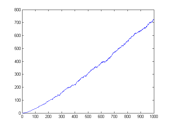
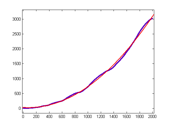
Let dx(n) denote (yx(n)-zx(n))/n. A quadratic least-squares fit of (Λ◦d(4))◦d(4) versus x for x=2, 3, 4, ..., 2000 is;
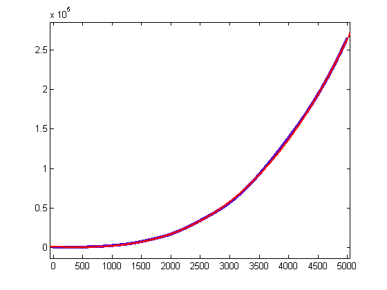
A cubic least-squares fit of -((Λ◦d(4))◦d(4))◦d(4) versus x for x=2, 3, 4, ..., 5000 is;
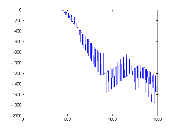
Let ck(n) denote Ramanujan's sum. A plot of ∑i=1x(ck([x/i])+1)(yi(n)-zi(n)) for k=17, n=50, and x=2, 3, 4, ..., 1500 is;
A plot of Σi=1x(n[x/i]-m[x/i])M(i) versus x for x=2, 3, 4, ..., 5000 is;
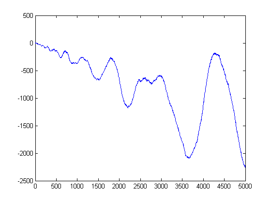
A plot of Σi=1x(m[x/i]-n[x/i]+1/6)M(i) versus x for x=2, 3, 4, ..., 5000 is;
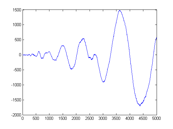
A plot of Σi=1xM([x/i])M(i) versus x for x=2, 3, 4, ..., 4000000 is;
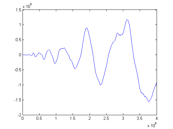
A plot of log(x!) (computed using Stieltjes' approximation) and |Σi=1xM([x/i])M(i)| versus x for x=2, 3, 4, ..., 100000 is;
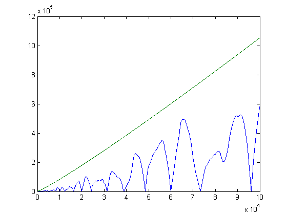
The oscillations of Σi=1xM([x/i])M(i) appear to be due to the first non-trivial zero of the zeta function. (Haselgrove used Ingham's smoothing function to disprove the Pólya conjecture and gives the corresponding smoothing function for the Merten's conjecture.) A plot of x(log(x))2 and |Σi=1xM([x/i])M(i)| versus x for x=2, 3, 4, ..., 2000000 is;
A plot of Σi=1xM([x/i])2 and Σi=1x(m[x/i]-n[x/i]+1/6)M([x/i]) versus x for x=2, 3, 4, ..., 5000 is;
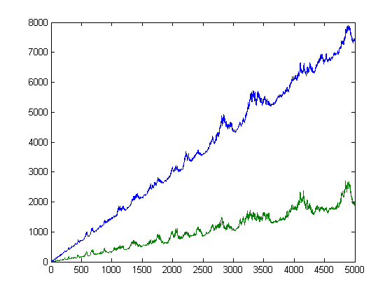
(43/30)+Σi=1x(m[x/i]-n[x/i]+1/6)M([x/i])≥(1/5)Σi=1xM([x/i])2. (11/300)+Σi=1x(m[x/i]-n[x/i]+1/6)2≥(1/25)Σi=1xM([x/i])2.
A plot of Σi=1xm[x/i]M(i) versus x for x=2, 3, 4, ..., 5000 is;
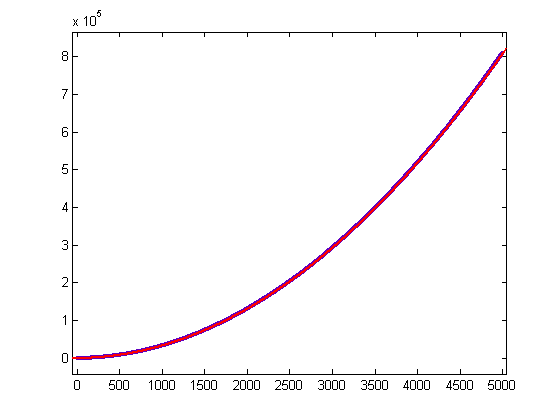
For a quadratic least-squares fit of Σi=1xm[x/i]M(i) versus x for x=2, 3, 4, ..., 5000, p1=0.03205 with a 95% confidence interval of (0.03205, 0.03205), p2=1.317 with a 95% confidence interval of (1.297, 1.337), p3=-29.2 with a 95% confidence interval of (-50.44, -7.957), SSE=3.25e+8, R-square=1, and RMSE=255.1.
Based on empirical evidence, ([x/n]([x/n]+1))/2≥-Σi=1[x/(j+1)]sgn(M([x/i]))i≥0, j=1, 2, 3, ..., where n=2+Σi=1j|sgn(M(i))|. A plot of ([x/n]([x/n]+1))/2+Σi=1[x/(j+1)]sgn(M([x/i]))i for j=1 and x=2, 3, 4, ..., 1000 is;
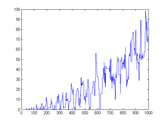
([x/n]([x/n]+1))/2 equals -Σi=1[x/(j+1)]sgn(M([x/i]))i in 194 instances. Let k=Σi=1j|sgn(M(i))| and let r=(k-1)-[(k-1)/4]4. Let d=2, 3, 3, or 4 when r=0, 1, 2, or 3 respectively. Based on empirical evidence, 1+([x/n]([x/n]+1))/2≥-Σi=1[x/(j+1)]sgn(M([x/i]))σ1(i)≥0, j=1, 2, 3, ..., where n=3[(k-1)/4]+d. A plot of 1+([x/n]([x/n]+1))/2+Σi=1[x/(j+1)]sgn(M([x/i]))σ1(i) for j=3 and x=2, 3, 4, ..., 200 is;
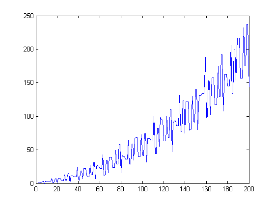
A plot of (1/x)Σi=1[x/10]σ1(i) versus x for x=2, 3, 4, ..., 200 is;
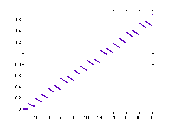
A plot of -(1/x)Σi=1[x/10]sgn(M([x/i]))σ1(i) versus x for x=2, 3, 4, ..., 200 is;
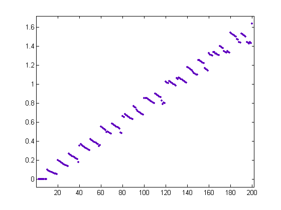
A plot of (1/x)Σi=1[x/10]|sgn(M([x/i]))|σ1(i) versus x for x=2, 3, 4, ..., 200 is;

A plot of (1/x)Σi=1[x/40]σ1(i)-(1/x)Σi=1[x/40]|sgn(M([x/i]))|σ1(i) versus x for x=2, 3, 4, ..., 300 is;
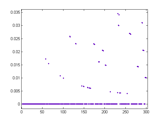
The bottom arc of values corresponds to x values where M(x)=0. A plot of (1/x)Σi=1[x/100]σ1(i)-(1/x)Σi=1[x/100]|sgn(M([x/i]))|σ1(i) versus x for x=2, 3, 4, ..., 500 is;
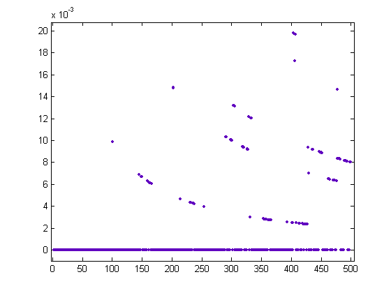
A plot of (1/x)Σi=1[x/200]σ1(i)-(1/x)Σi=1[x/200]|sgn(M([x/i]))|σ1(i) versus x for x=2, 3, 4, ..., 2000 is;
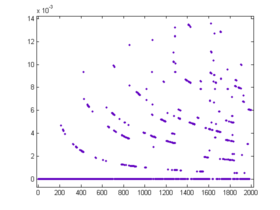
A table of the x, M(x), (1/x)Σi=1[x/200]σ1(i)-(1/x)Σi=1[x/200]|sgn(M([x/i]))|σ1(i) (denoted by "delta sums"), (1/x)Σi=1[x/200]σ1(i) (denoted by "sigma sum"), and (1/x)Σi=1[x/200]σ1(i)/((1/x)Σi=1[x/200]σ1(i)-(1/x)Σi=1[x/200]|sgn(M([x/i]))|σ1(i)) (denoted by "ratio") values associated with the different arcs is;
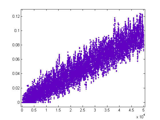
A plot of eγΣi=1[x/50]|sgn(M([x/i]))|i-Σi=1[x/50]|sgn(M([x/i]))|σ1(i) versus x for x=2, 3, 4, ..., 1000 is;
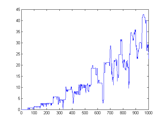
A plot of eγΣi=1[x/1000]|sgn(M([x/i]))|i-Σi=1[x/1000]|sgn(M([x/i]))|σ1(i) versus x for x=2, 3, 4, ..., 10000 is;
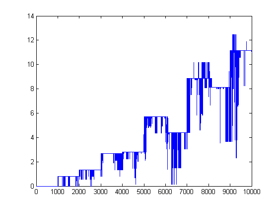
A plot of √Σi=1[x/2]|sgn(M([x/i]))|-√-Σi=1[x/2]sgn(M([x/i])) versus x for x=2, 3, 4, ..., 10000 is;
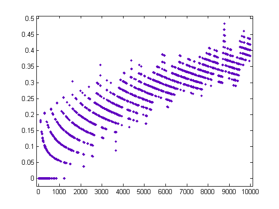
Let d(2)=0 and let d(3), d(4), d(5), ..., d(14) equal 1, 0, 0, 1, 1, 0, 1, 1, 1, 1, 1, and 1 respectively. Let d(x+12)=d(x)+1. The loss in value of Σi=1[x/4]sgn(M([x/i]))i (compared to Σi=1xsgn(M([x/i]))i) is [(x+1)/2] (due to the M(1) term being effectively set to 0) minus d(x) (due to the M(3) term being effectively set to 0). d(x) appears to be related to h(x); d(x)+h(x), x=2, 3, 4, ..., equals 0, 1, 1, 1, 1, 2, 2, 2, 2, 3, 3, 3, 3, 4, 4, 4, 4, ..... Let e(2)=e(3)=0 and e(4), e(5), e(6), ..., e(23) equal 1, 0, 0, 0, 1, 1, 0, 0, 1, 1, 1, 0, 1, 1, 1, 1, 1, 1, 1, and 1 respectively. Let e(x+20)=e(x)+1. e(x) is the gain in value due to effectively setting M(4) to 0. Let q(2)=q(3)=0 and q(4), q(5), q(6), ..., equal 1-e(4), 1-e(5), 1-e(6), 1-e(7), 1-e(8), 2-e(9), 2-e(10), 2-e(11), 2-e(12), 2-e(13), 3-e(14), 3-e(15), 3-e(16), 3-e(17), 3-e(18), .... A plot of Σi=1xsgn(n[x/i]-m[x/i])-q(x) versus x for x=2, 3, 4, ..., 2000 is;
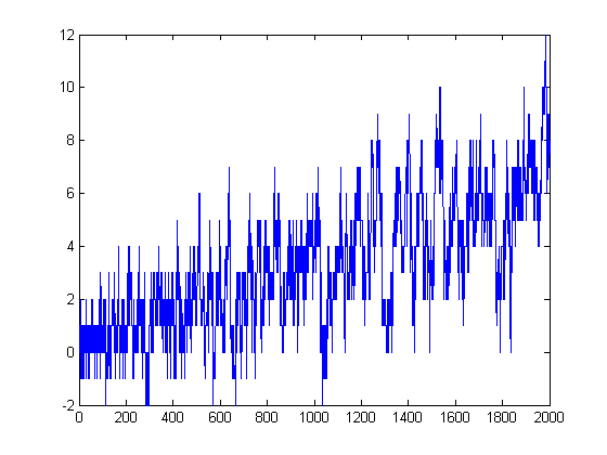
For x≤10250, 2+Σi=1xsgn(n[x/i]-m[x/i])≥q(x). Let f(2)=f(3)=f(4)=0 and f(5), f(6), f(7), ..., f(34) equal 1, 0, 0, 0, 0, 1, 1, 0, 0, 0, 1, 1, 1, 0, 0, 1, 1, 1, 1, 0, 1, 1, 1, 1, 1, 1, 1, 1, 1, and 1 respectively. Let f(x+30)=f(x)+1. f(x) is the gain in value due to effectively setting M(5) to 0. Let r(2)=r(3)=r(4)=0 and r(5), r(6), r(7), ..., equal 1-f(5), 1-f(6), 1-f(7), 1-f(8), 1-f(9), 1-f(10), 2-f(11), 2-f(12), 2-f(13), 2-f(14), 2-f(15), 2-f(16), 3-f(17), 3-f(18), 3-f(19), 3-f(20), 3-f(21), 3-f(22), .... r(x) is less than or equal to q(x).
Let b(2), b(3), b(4), ..., b(7) equal 1, 0, 1, 1, 1, and 1 respectively. Let b(x+6)=b(x)+1. Let c(2), c(3), c(4), ..., equal 1-b(2), 1-b(3), 1-b(4), 2-b(5), 2-b(6), 2-b(7), 3-b(8), 3-b(9), 3-b(10), .... A plot of Σi=1xsgn(M([x/i]))-c(x) versus x for x=2, 3, 4, ..., 1000 is;
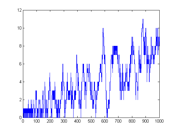
Σi=1xsgn(M([x/i])) equals c(x) in 66 instances. h(x)-c(x) equals -1, 0, or 1.
Let L(x) denote Σi=1xλ(i) where λ(i) is the Liouville function. Σd|nλ(d) equals 1 if n is a perfect square or 0 otherwise. Replacing φ(j) with λ(j) in the T matrix (defined in the summary) gives L(x)=Σi is perfect squareM([x/i]). A plot of L(x) and -Σi is perfect square(n[x/i]-m[x/i]) versus x for x=2, 3, 4, ..., 10250 is;
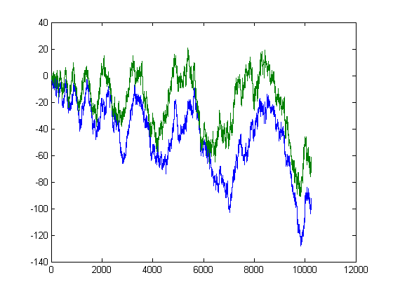
A plot of L(x) and Σi is perfect square(m[x/i]-n[x/i]+1/6) versus x for x=2, 3, 4, ..., 10000 is;
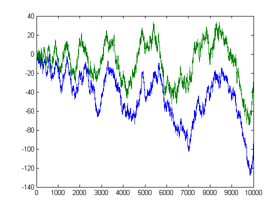
A plot of L(x) and -Σi is perfect square(n[x/i]-m[x/i]) versus x for x=2, 3, 4, ..., 50000 is;
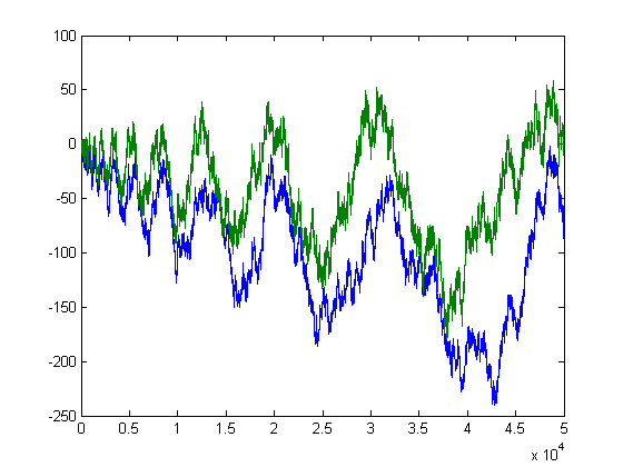
A plot of -Σi=1xM([x/i])L(i) and x3/2/6 versus x for x=2, 3, 4, ..., 50000 is;
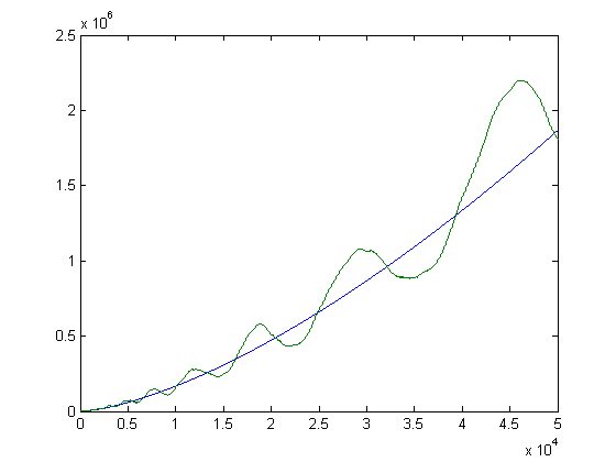
A plot of √Σi=1xM([x/i])L(i)2 and x/3 versus x for x=2, 3, 4, ..., 50000 is;
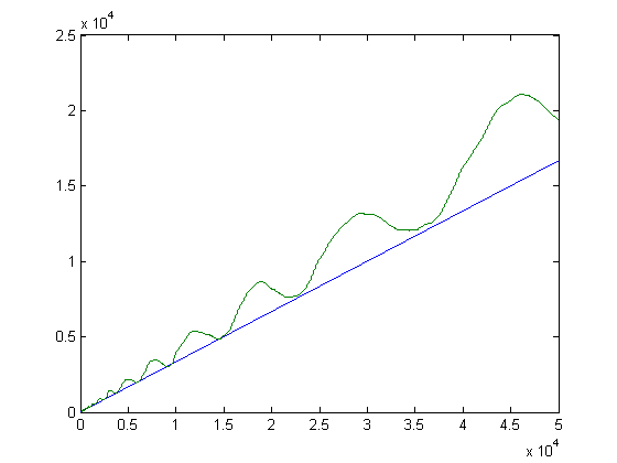
A plot of -Σi=1xM([x/i])2L(i) and x3/2/2 versus x for x=2, 3, 4, ..., 50000 is;
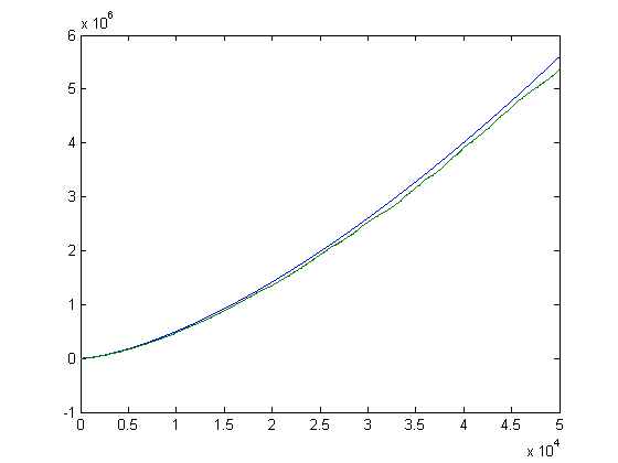
x3/2/2 is greater than or equal to -Σi=1xM([x/i])2L(i). A plot of √Σi=1xM([x/i])2L(i)2 and x/2 versus x for x=2, 3, 4, ..., 50000 is;
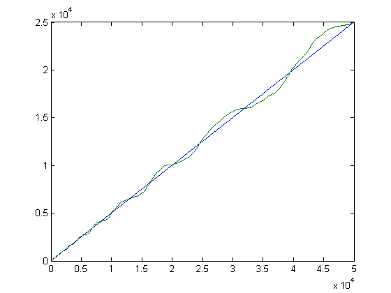
A plot of -Σi=1xL(i) and x3/2/2 versus x for x=2, 3, 4, ..., 50000 is;
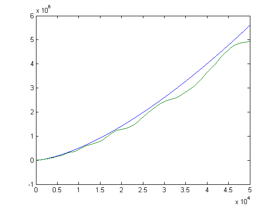
A plot of √Σi=1xL(i)2 and x/2 versus x for x=2, 3, 4, ..., 50000 is;
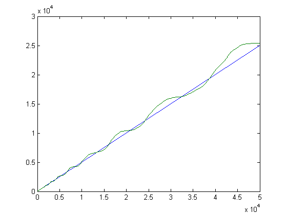
A plot of -Σi=1xM([x/i])log(i)L(i) and 2x3/2 versus x for x=2, 3, 4, ..., 50000 is;
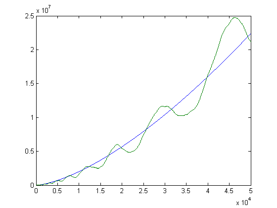
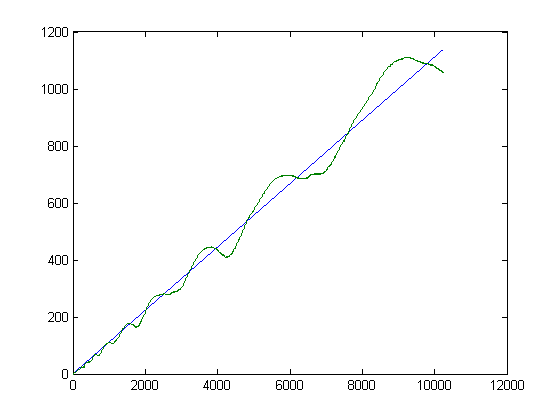
-12Σi=1xM([x/i])L(i) is greater than or equal to -Σi=1xM([x/i])log(i)L(i). A plot of √Σi=1x(n[x/i]-m[x/i])2L(i)2 and x/9 versus x for x=2, 3, 4, ..., 10250 is;
Software
A C program for computing various functions of mx and nx for x up to 10250 is test1bd. Subroutines used are mertens8, lagrang1, haros5, numdiv, liouville, and table2 . A C program for computing the Mertens function, Σi=1xsgn(M([x/i])), or Σi=1xsgn(M([x/i]))i is mtestsy. A C program for computing the Mertens function, Σi=1x|sgn(M([x/i]))|, or Σi=1x|sgn(M([x/i]))|i is mtestsx. A C program for computing Σi=1xM([x/i])2 is mtest7. A C program for computing h(x), q(x), and c(x) is test20f. A C program for computing functions of L(x) is mtest7b. Subroutines used are liouvill, dirchar, and mangoldt. A C program for computing U(x)-L(x) is test1r1. A subroutine used is euclid.
A C program for computing functions of mx and nx for x up to 50000 is test1bf. Other subroutines used are mertens9 and dirchar. A C program for computing functions of ox and px is test1bg. A subroutine used is mertensf. A C program for computing functions of qx and rx is test1bh. A subroutine used is mertense. A C program for computing functions of sx and tx is test1bi. A subroutine used is mertensg. A C program for computing functions of ux and vx is test1bj. A subroutine used is mertensh. Similar programs and subroutines are test1bk, mertensm, test1bl, mertensk, test1bm, mertenso, test1bn, and mertensi. A C program for computing functions of yx(n) and zx(n) is test1bz. Subroutines used are mertenax, haros6, and lagrange2. A C program for computing yx(n) and zx(n) for large n is test1bap. Subroutines used are mertenau, haros9, add64, sub64, div12864, and mul6464. A C program for computing yx(n) and zx(n) for smaller n is test1bax. Subroutines used are mertenav and haros8. A C program for computing functions of interpolated differences in numbers of fractions is test5. A subroutine used is interp. A C program for computing functions of interpolated approximate differences in numbers of fractions is test6. A subroutine used is interp1. "include" files are output2, output4, and output5. A C program for computing functions of yx(n) and zx(n) involving Ramanujan's sum and Gauss sums associated with Dirichlet characters is test1bz1. Subroutines used are mertenaw, haros7, mobius, gauss, and ramanuj. A C program for computing ∑i=1xM(x/i)2 where i|x is test1bze. A subroutine used is newmob. A C program for computing measures of local maxima is test20m. A C program for computing ∑i=1x|M(x/i)| where i|x is test1bzf. A C program for computing measures of local maxima is test21m. A C program for computing M(x) for large x is test19b. Subroutines used are sumlo and sumhi. C programs for computing various maxima for x up to 1000000000 are test1bzq, test1bzr, test1bzs, test1bzt, test1bzu, test1bzv, and test1bzw. A C program for computing maxima for the σ0(x) function for large x is test1ac. A C program for computing j(x) for maxima based on the σ0(x) function for large x is test1ag. Subroutines used are nuriv, nuhic, nuloc, newmob, div6432, mul6432, sub64, lmbd, and carry. A corresponding C program with more dynamic range is test1af. Subroutines used are newriv, newhic, newloc, and div12864. A more efficient C program with more dynamic range is test1ah. Subroutines used are fastriv, fasthic, fastloc, and div6464. A C program for computing j(x) for maxima based on the σ0(x) function for large x is test1ar. This program uses more RAM and requires a 64-bit OS. Subroutines used are newmobl, newrivl, newhicl, newlocl, and table3. A C program for computing maxima based on j(x) is test1ap. This program uses more RAM and requires a 64-bit OS. A program for computing j(x) for highly composite numbers is test1ar9. Subroutines used are newhicl9, newlocl9, newrivl9, newmobl9, primed, and tablel9. OpenMP was used to do parallel processing on an Intel i7-6700K CPU with 64 GB of RAM. A more efficient subroutine (less amenable to parallel processing) is newhicla. An algorithm for computing the Mertens function on a GPU (a simplistic version of Kuznetsov's algorithm) is test19g. A C program for computing ∑i=1xM([x/i])2 where x is a highly composite number is test1asp. A subroutine used is newmert. OpenMP is used to do parallel processing. The algorithm is also amenable to processing on a NVIDIA Tesla C2070™ GPU. A C program for computing j(x) where x is a highly composite number is test1arp. Computing j(x) for highly composite numbers up to about 100 quadrillion is practical. A CUDA C program for computing j(x) where x is a highly composite number is test1arc. Another C program for computing j(x) where x is a highly composite number is test1arq. Computing j(x) for highly composite numbers up to about 1018 is practical. Another C program for computing ∑i=1xM([x/i])2 where x is a highly composite number is test1asr. OpenMP is used to do parallel processing. Computing ∑i=1xM([x/i])2 for highly composite numbers up to about 1017 is practical.
z Transform of M([x/i])
A plot of M([x/1]), M([x/2]), M([x/3]), ..., M([x/x]) for x=500000 is;
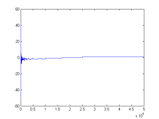
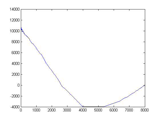
In general, the z transform of this sequence appears to be stable and causal (the initial value theorem appears to be applicable). A plot of the autocorrelation of M([x/i]) versus the shift amount for x=8000 is;
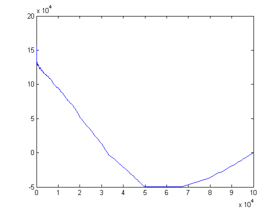
A plot of the autocorrelation of M([x/i]) versus the shift amount for x=100000 is;
Farey Sequences
The Farey sequence Fn of order n is the ascending sequence of irreducible fractions between 0 and 1 whose denominators do not exceed n. Fractions can be mapped to a two-dimensional coordinate system. In the integer lattice, let the numerators of fractions be along the x axis and the denominators be along the y axis. The polygon generated by a Farey sequence of order 11 is;
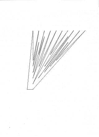
There are no interior lattice points, so the area of the polygon is 1/2 the number of fractions minus 1 (by Pick's theorem that A(P)=½B+I-1). For reduced fractions less than or equal to 1, the simple polygon generated by a Farey sequence has the maximum possible perimeter-to-area ratio. For Farey sequences of orders 2, 3, 4, ..., and 100, the average length of a side of the polygon plotted against the order is;
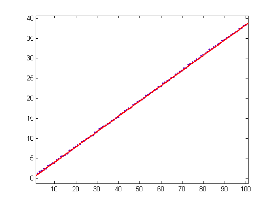
For a linear least-squares fit (where f(x)=p1x+p2), p1=0.3815 with a 95% confidence interval of (0.3807, 0.3823) and p2=0.2376 with a 95% confidence interval of (0.1904, 0.2848). SSE=1.298, R-square=0.9999, adjusted R-square=0.9999, and RMSE=0.1157. Multiple-word arithmetic subroutines used to accurately compute the lengths are nword and sqrtn. A driver for the subroutines is test1a. A program for computing the average lengths and the average square roots of the lengths without using multiple-word arithmetic is test6f. A program for generating a Farey sequence using Lagrange's algorithm is lagrange. For Farey sequences of orders 2, 3, 4, ..., 600, the average of the square roots of the lengths plotted against the square root of the order is;
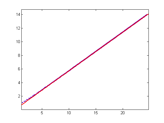
For a linear least-squares fit, p1=0.5684 with a 95% confidence interval of (0.5682, 0.5687) and p2=0.04928 with a 95% confidence interval of (0.04479, 0.05376). SSE=0.2032, R-square=1, adjusted R-square=1, and RMSE=0.01845.
Franel and Landau proved that the Riemann hypothesis is equivalent to the statement Σk≤Φ(x)|rk-k/Φ(x)|<<x½+ε for all ε>0 as x→∞. (rk denotes a fraction in a Farey sequence of order x [excluding 0/1] and Φ(x) denotes the number of fractions.) For x=2, 3, 4, ..., and 600, a plot of the sums versus √x is;
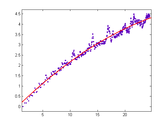
For a quadratic least-squares fit, p1=-0.003322 with a 95% confidence interval of (-0.003701, -0.002943), p2=0.2605 with a 95% confidence interval of (0.2491, 0.272), and p3=-0.0964 with a 95% confidence interval of (-0.1761, -0.01671) . SSE=15.19, R-square=0.9719, adjusted R-square=0.9718, and RMSE=0.1597. Multiple-word arithmetic is not used. A program for computing the sums is test1b. A plot of (Φ(x)Σk≤Φ(x)(rk-k/Φ(x))2)½ versus √x for x=2, 3, 4, ..., 600 is;
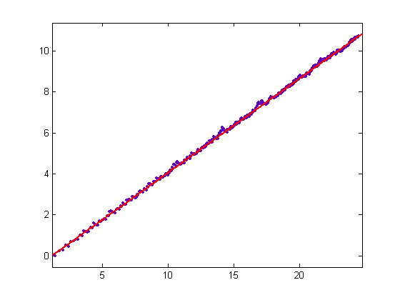
For a linear least-squares fit, p1=0.4589 with a 95% confidence interval of (0.4579, 0.4599) and p2=-0.5259 with a 95% confidence interval of (-0.5437, -0.5081). SSE=3.204, R-square=0.9992, adjusted R-square=0.9992, and RMSE=0.07326. This plot superimposed on the plot of the average square roots of the lengths of the sides of the polygon is;
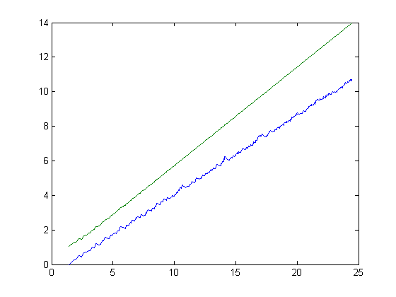
On page 267 of H. M. Edwards' Riemann's Zeta Function, the inequality Σ|δv|≤(AΣδv2)½<K½x(½)+ε (an implication of the Riemann hypothesis) is given. K is a constant depending on ε. Apart from the notation, (AΣδv2)½ is the same quantity as given in the first of the above two plots. Based on the above plot, some constant multiple of K½x(½)+ε would be greater than the average square roots of the lengths of the sides of the polygon.
On page 265 of Edwards' book, the inequality M(x)≤2πΣ Av=1|δv| is given. (Σ|δv|=o(x(½)+ε) implies the Riemann hypothesis.) Comparing the second and third plots above, the average of the square roots of the lengths of the sides of the polygon is greater than Σ|δv| (and some constant multiple of the average of square roots is greater than 2πΣ|δv|).
The above plot superimposed on the plot of sums (Σ|δv|) is;
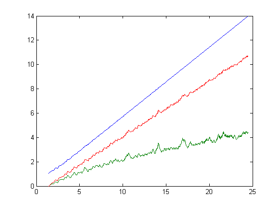
This plot indicates that a line can be drawn, bounded above by the first "curve" and below by the second "curve" and without intersecting either of the "curves". (Σ|δv| is less than or equal to (AΣδv2)½ by the Schwarz inequality.) This is relevant to the Stieltjes hypothesis. The corresponding plot for x=2, 3, 4, ..., 50 (showing the relationship between the "curves" in more detail) is;
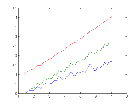
The two greatest lengths of a side of the polygon are √(x-1)2+(x-2)2) and √(x-1)2+1. The average square root of the lengths is then less than √x. The "curve" of average square roots of the lengths is then bounded above with a line having a slope of 1. It remains to be shown that the "curve" of average square roots of the lengths of the sides of the polygon is above the "curve" (AΣδv2)½. The "curve" of average square roots of the lengths is essentially a straight line when plotted against √x due to the formula M(x)=Σe2πir where rv is a fraction in the Farey sequence and M(x) is the Mertens function (as x gets large, the sum of the lengths of chords of the unit circle approaches the circumference of the circle).
The assumption in using the measure δv in the Franel-Landau theorem is that the Farey sequence is too erratic to analyze. This isn't entirely the case in that the Farey sequence can be analyzed statistically. A plot of the sum of cos(2πrv) starting from 1/4 and proceeding in opposite directions to 0/1 and 1/2 for x=35 is;
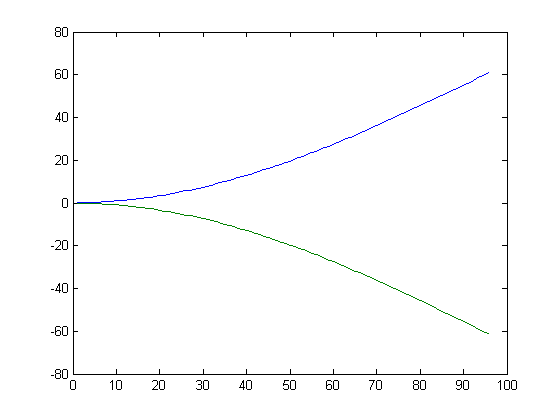
For a quadratic least-squares fit of one of these curves, the R-square value is typically greater than 0.99. A different pair of quadratic curves corresponds to every x value and the three parameters p1, p2, and p3 of the curves change in a fairly predictable manner. A plot of p1 (for the upper curve) for x=10, 11, 12, ..., 55 is;
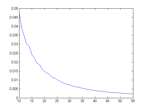
The corresponding plot for p2 is;
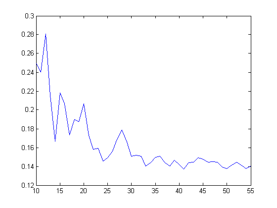
The corresponding plot for p3 is;

The following is a partial explanation for the relationship between the curve of M(x) values and the curve of mx-nx values. A program for computing a Farey sequence from a half-order sequence is test1o (when the order is odd, a half-order of (x+1)/2 is used). A subroutine used is lagrang1. (For details on how the algorithm works, see the section "Generating Farey Series Using Integer Lattice Theorems" in the link farey.) Fractions in the full-order sequence are generated by interpolating between fractions in the half-order sequence. A remarkable property of the Farey sequence is that the corresponding interpolation of sums of cosines is almost linear. (For example, for x=29 [the half-order], the interpolated fractions between 7/25 and 2/7 are 16/57, 9/32, 11/39, 13/46, and 15/53 and the respective sums of cosines [starting with the sum for 7/25] are 155.3513, 155.1596, 154.9645, 154.7645, 154.5610, 154.3551, and 154.1325.) The change in the value of the Mertens function from the half-order Farey sequence to the full-order sequence is then mostly dependent on the change in the number of fractions. A program for confirming this is test1pa. Let ax denote the sum of cos(2πrv) for rv up to 1/4 and bx denote the sum of cos(2πrv) for rv between 1/4 and 1/2. For example, a225=2455.446, m225=3858, b225=-2453.946, n225=3854, a450=9807.467, m450=15405, b450=-9810.967, and n450=15410. Then a450(m225/m450)=2456.164, b450(n225/n450)=-2453.6966 and the sum of these two quantities is 2.4674, close to the expected value of 1.5.
A program for computing an upper and lower bound of the number of fractions before 1/4 or after 1/4 (using the ceiling and floor functions) is test1ra. A plot of the upper bounds, lower bounds, and numbers of fractions before 1/4 for x=2, 3, 4, ..., 75 is;
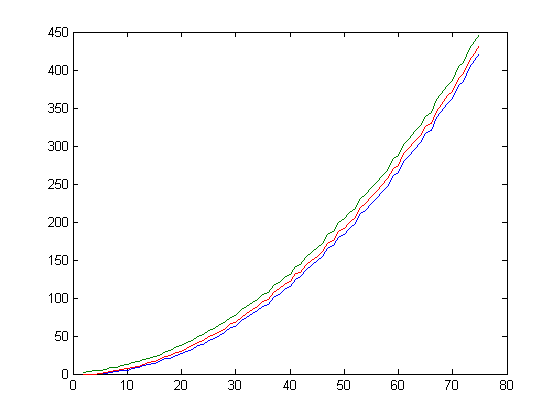
A plot of the upper bounds, lower bounds, and numbers of fractions after 1/4 for x=2, 3, 4, ..., 75 is;

A plot of half the absolute value of the Mertens function and the square root of the upper bound minus the lower bound for x=2, 3, 4, ..., 500000 is;
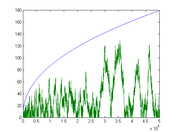
A quadratic-least square fit of the square root of the upper bound minus the lower bound plotted against √x for x=2, 3, 4, ..., 900 is;
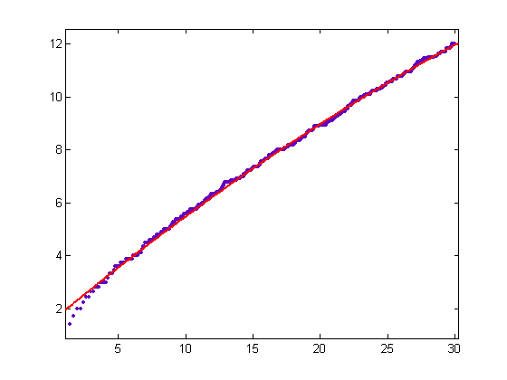
p1=-0.002466 with a 95% confidence interval of (-0.002563, -0.002369), p2=0.4227 with a 95% confidence interval of (0.4191, 0.4263), and p3=1.501 with a 95% confidence interval of (1.47, 1.531). SSE=5.14, R-square=0.999, adjusted R-square=0.999, and RMSE=0.07574.
A quadratic least-squares fit of the square root of the upper bound minus the lower bound plotted against √x for x=2, 3, 4, ..., 2000 is;
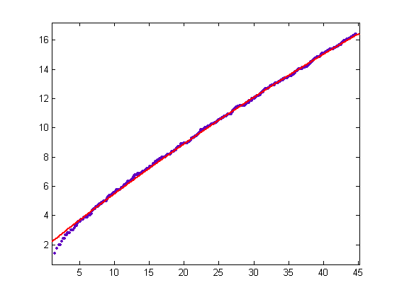
p1=-0.001162 with a 95% confidence interval of (-0.001193, -0.00113), p2=0.3756 with a 95% confidence interval of (0.3739, 0.3773), and p3=1.847 with a 95% confidence interval of (1.825, 1.869). SSE=13.39, R-square=0.9994, adjusted R-square=0.9994, and RMSE=0.08191. The curve becomes more linear as x increases, indicating that the Stieltjes hypothesis is true.
A plot of πΣ|δv|, (3π/4)Σ|δv|, (π/2)Σ|δv|, half the absolute value of the Mertens function, and the square root of the upper bound minus the lower bound for x=2, 3, 4, ..., 1812 is;
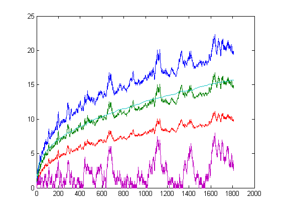
The square root of the upper bound minus the lower bound is then of utility in determining if Σ|δv|=O(x½) (despite the origin of the definition of the upper and lower bounds). A rigorous proof that the difference between the upper bound and the lower bound increases linearly (mostly) with x depends on the following property of the φ function; 4 divides φ(n) if and only if n has a prime factor of the form 4k+1, 8 divides n, 4 divides n and n has an odd prime factor, or n has at least two distinct prime factors of the form 4k+3. 4 doesn't divide φ(n) if n is a power of a prime of the form 4k+3 or twice a power of a prime of the form 4k+3. The upper bound minus the lower bound then equals 3+Σ[logq(x)]+Σ[logq(x/2)] where the summation is over the primes q of the form 4k+3 that are less than or equal to x (the brackets denote the floor function). (Of course, x is greater than this sum so that when the square roots of the upper bounds minus the lower bounds are plotted against √x, the "curve" is bounded above with a line having a slope of 1.)
On page 264 of Edwards' book, the formula Σv=1A(x)f(rv)=Σk=1∞Σj=1kf(j/k)M(x/k) is given. The function f(u)=e2πiu is used to find a relationship between the Mertens function and Σv=1A(x)|δv|. The function {(φ(d)-[φ(d)/4]4)/φ(d)}/φ(d) where d denotes the denominator of a fraction, the curly brackets denote the ceiling function, and the brackets denote the floor function can be used to find a direct relationship between the Mertens function and the square root of the upper bound minus the lower bound. A program for confirming that the sum of this function equals the upper bound minus the lower bound is test1b4. Subroutines used are euler and euclid. Substituting the function into the right-hand side of the above formula and using the floor of x/k gives a useable result. Let N(x) denote -Σi=1xM([x/i])i{(φ(i)-[φ(i)/4]4)/φ(i)}/φ(i). A plot of √N(x), the square root of the upper bound minus the lower bound, and half the absolute value of the Mertens function for x=2, 3, 4, ..., 1280 is;
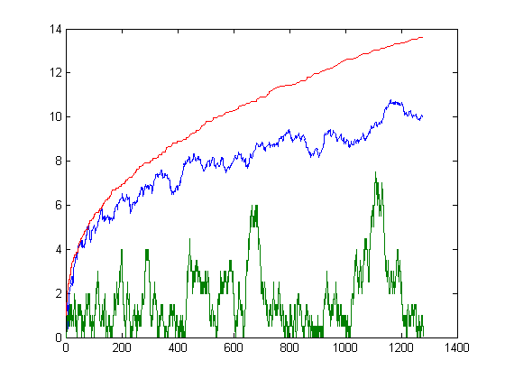
A program for computing N(x) is test1b6. Subroutines used are mertens1 and haros2. A linear least-squares fit of N(x) versus √x for x=2, 3, 4, ..., 5128 is;
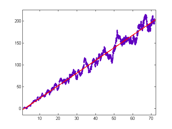
p1=2.892 with a 95% confidence interval of (2.875, 2.909) and p2=-5.61 with a 95% confidence interval of (-6.476, -4.745). SSE=5.675e+5, R-square=0.9555, adjusted R-square=0.9555, and RMSE=10.52. N(x) is analogous to the quantity (AΣδv2)½. A plot of N(x) and 2π(AΣδv2)½ versus √x for x=2, 3, 4, ..., 1280 is;
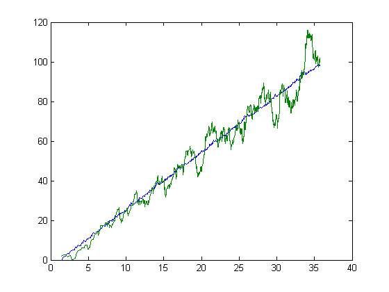
For a linear least-squares fit of 2π(AΣδv2)½ versus √x for x=2, 3, 4, ..., 2560, p1=2.854 with a 95% confidence interval of (2.852, 2.856) and p2=-2.776 with a 95% confidence interval of (-2.845, -2.708). SSE=892.5, R-square=0.9997, adjusted R-square=0.9997, and RMSE=0.5908.
Σi=1xM([x/(in)])=1 for n=1, 2, 3, ..., x. Usually, M([x/i]) is negative for i=2, 3, 4, ..., [x/2] (the first exception to this is for x=188). Let m denote the largest absolute value of M([x/i]) where 4 does not divide φ(i) and i≤[x/2]. If the sign of M([x/i]) doesn't change (that is, become positive), then mx/(x-1)/2 is greater than N(x). A program for determining sign changes of M([x/i]) is test1b7. Except for small M([x/i]) values (say less than 4), the estimated M([x/i]) value (for positive M([x/i]) values) computed from M(x) using the numbers of fractions in the Farey sequences before and after 1/4 (as in half-orders discussed above) is accurate enough to compute the correct sign of M([x/i]). A program for confirming this is test1b5. A subroutine used is mertens. The next step is to use 0 (instead of M(x)) as the initial value from which to estimate M([x/i]) values. Let P(x) denote these values. A plot of P(x) versus √x for x=2, 3, 4, ..., 1280 is;
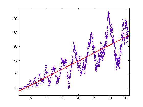
The problem then becomes that of determining if P(x) is greater than 0 and less than the upper bounds minus the lower bounds. A program for computing P(x) is test1b8. A subroutine used is mertens2. A plot of P(x) and the upper bounds minus the lower bounds versus √x for x=2, 3, 4, ..., 5128 is;
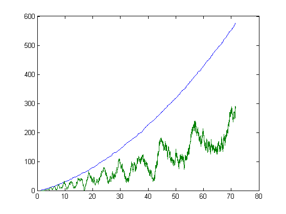
Let L(x) denote Σi=1xax(m[x/i]/mx) and R(x) denote Σi=1xbx(n[x/i]/nx). A plot of L(x) and R(x) for x=2, 3, 4, ..., 1280 is;
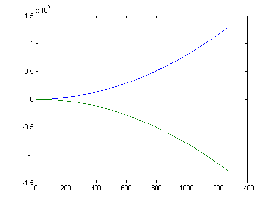
For a quadratic least-squares fit of L(x), p1=0.07958 with a 95% confidence interval of (0.07958, 0.07958), p2=-0.318 with a 95% confidence interval of (-0.3189, -0.3171), and p3=-0.6552 with a 95% confidence interval of (-0.9089, -0.4014). SSE=3005, R-square=1, adjusted R-square=1, and RMSE=1.535. For a quadratic least-squares fit of R(x), p1=-0.07958 with a 95% confidence interval of (-0.07958, -0.07958), p2=0.2144 with a 95% confidence interval of (0.2132, 0.2155), and p3=-0.7061 with a 95% confidence interval of (-1.034, -0.378). SSE=5026, R-square=1, adjusted R-square=1, and RMSE=1.985. A program and subroutines for computing these quantities are test1b9, mertens3, and haros3. A quadratic least-squares fit of L(x) for x=2, 3, 4, ..., 101 is;
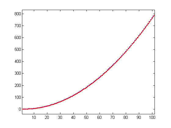
p1=0.07973 with a 95% confidence interval of (0.07962, 0.07985), p2=-0.3372 with a 95% confidence interval of (-0.3493, -0.325), and p3=-0.1597 with a 95% confidence interval of (-0.4305, 0.1112). SSE=17.81, R-square=1, adjusted R-square=1, and RMSE=0.4285. L(x) and R(x) appear to have fixed probability distributions.
Let S(x) denote Σi=1xax(m[x/i]/mx)i and T(x) denote Σi=1xbx(n[x/i]/nx)i. A plot of √S(x) and √-T(x) for x=2, 3, 4, ..., 900 is;
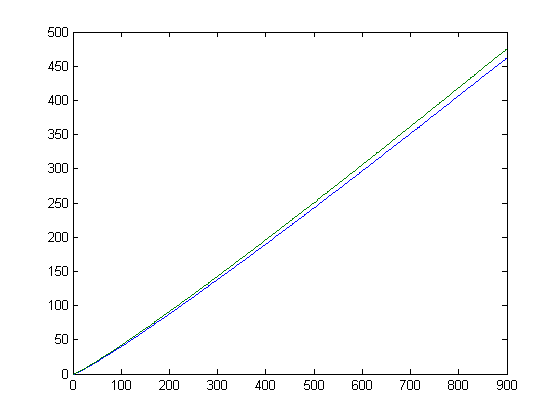
For a quadratic least-squares fit of √S(x), p1=6.415e-5 with a 95% confidence interval of (6.293e-5, 6.537e-5), p2=0.4654 with a 95% confidence interval of (0.4642, 0.4665), and p3=-6.677 with a 95% confidence interval of (-6.899, -6.456). SSE=1125, R-square=0.9999, adjusted R-square=0.9999, and RMSE=1.12. For a quadratic least-squares fit of √-T(x), p1=6.271e-5 with a 95% confidence interval of (6.152e-5, 6.39e-5), p2=0.4809 with a 95% confidence interval of (0.4798, 0.482), and p3=-6.305 with a 95% confidence interval of (-6.521, -6.088). SSE=1079, R-square=0.9999, adjusted R-square=0.9999, and RMSE=1.097. These parameters change somewhat for different upper bounds of x.
A plot of Σi=1xa[x/i] and Σi=1xb[x/i] for x=2, 3, 4, ..., 900 is;
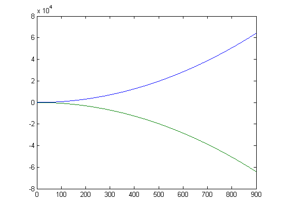
For a quadratic least-squares fit of Σi=1xa[x/i], p1=0.07958 with a 95% confidence interval of (0.07958, 0.07958), p2=-0.4207 with a 95% confidence interval of (-0.4207, -0.4207), and p3=0.3923 with a 95% confidence interval of (0.3901, 0.3945). SSE=0.1076, R-square=1, adjusted R-square=1, and RMSE=0.01096. For a quadratic least-squares fit of Σi=1xb[x/i], p1=-0.07958 with a 95% confidence interval of (-0.07958, -0.07958), p2=0.4207 with a 95% confidence interval of (0.4207, 0.4207), and p3=0.1077 with a 95% confidence interval of (0.1055, 0.1099). SSE=0.1077, R-square=1, adjusted R-square=1, and RMSE=0.01096. As expected, the values of these parameters are close to those of L(x) and R(x).
A plot of √Σi=1xia[x/i] and √-Σi=1xib[x/i] for x=2, 3, 4, ..., 900 is;
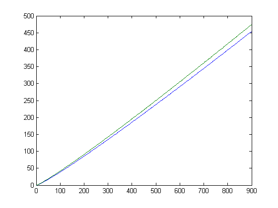
For a quadratic least-squares fit of √Σi=1xia[x/i], p1=6.544e-5 with a 95% confidence interval of (6.419e-5, 6.669e-5), p2=0.4553 with a 95% confidence interval of (0.4541, 0.4564), and p3=-6.825 with a 95% confidence interval of (-7.052, -6.597). SSE=1187, R-square=0.9999, adjusted R-square=0.9999, and RMSE=1.151. For a quadratic least-squares fit of √-Σi=1xib[x/i], p1=6.28e-5 with a 95% confidence interval of (6.16e-5, 6.4e-5), p2=0.4797 with a 95% confidence interval of (0.4786, 0.4808), and p3=-6.337 with a 95% confidence interval of (-6.554, -6.119). SSE=1086, R-square=0.9999, adjusted R-square=0.9999, and RMSE=1.101.
For a linear least-squares fit of √-½Σi=1xiM([x/i]) (where M(1) and M(3) are set to 0) for x=2, 3, 4, ..., 900, p1=0.1529 with a 95% confidence interval of (0.1528, 0.1529) and p2=0.06837 with a 95% confidence interval of (0.04627, 0.09047). SSE=25.43, R-square=1, adjusted R-square=1, and RMSE=0.1684. A plot of √-½Σi=1xiM([x/i]) for x=2, 3, 4, ..., 103 is;
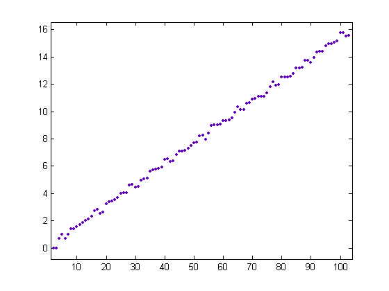
The values decrease if and only if x-6 is divisible by 12. A plot of √√-½Σi=1xiM([x/i]), the square root of the upper bound minus the lower bound, and half the absolute value of the Mertens function for x=2, 3, 4, ..., 2560 is;
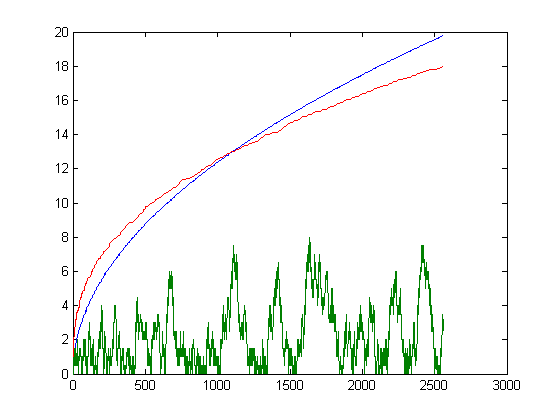
This plot indicates that √√-½Σi=1xiM([x/i]) will eventually become greater than πΣv=1A(x)|δv| (since 4/3 times the square root of the upper bound minus the lower bound is approximately equal to πΣv=1A(x)|δv|). Based on a linear least-squares fit of √-½Σi=1xiM([x/i]) for x=2, 3, 4, ..., 3626, p1=0.1529 and p2=0.0721. A plot of the estimated value of √√-½Σi=1xiM([x/i]) using these parameters, the square root of the upper bound minus the lower bound, and 4/3 times the square root of the upper bound minus the lower bound for x=2, 3, 4, ..., 40000 is;
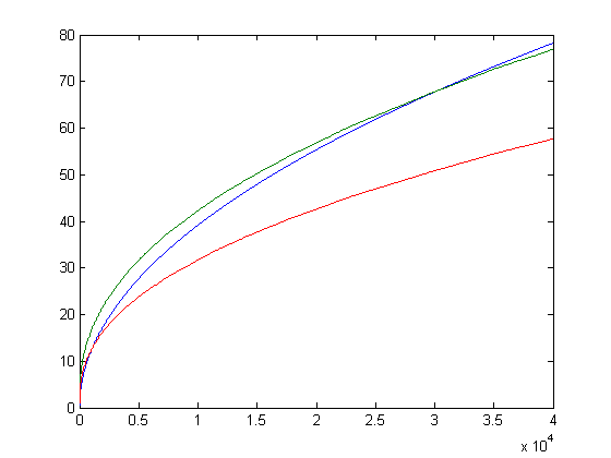
For a quadratic least-squares fit of Σi=1xm[x/i] where x=2, 3, 4, ..., 1812, p1=0.125 with a 95% confidence interval of (0.125, 0.125), p2=-0.5 with a 95% confidence interval of (-0.5001, -0.4999), and p3=.3217 with a 95% confidence interval of (0.2867, 0.3387). SSE=63.7, R-square=1, adjusted R-square=1, and RMSE=0.1877. For a quadratic least-squares fit of Σi=1xn[x/i], p1=0.125 with a 95% confidence interval of (0.125, 0.125), p2=-0.3333 with a 95% confidence interval of (-0.3334, -0.33321), and p3=0.1456 with a 95% confidence interval of (0.09968, 0.1915). SSE=197.9, R-square=1, adjusted R-square=1, and RMSE=0.3309. A plot of Σi=1xm[x/i]-n[x/i] for x=2, 3, 4, ..., 101 is;
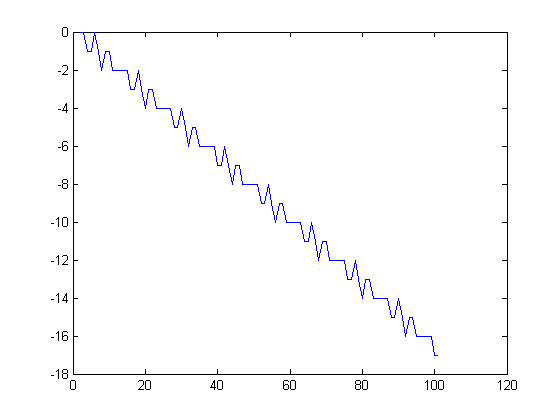
The slope and intercept of the negative of this quantity are about the same as those of √-½Σi=1xiM([x/i]) (the respective slopes are 1/6 and 0.1529). A program for computing the Mertens function up to x=2560 is test1ba. Subroutines used are mertens4 and haros4.
The rationale for setting M(1) and M(3) to 0 is that there is no possibility of a fraction being before 1/4 in these cases (no fractions being before 1/4 for M(4) is deemed to be acceptable). For a linear least-squares fit of √-½Σi=1xiM([x/i]) where M(1), M(3), M(4), and M(5) are set to 0 and x=2, 3, 4, ..., 1812, p1=0.1078 with a 95% confidence interval of (0.1078, 0.1079) and p2=0.04947 with a 95% confidence interval of (0.03317, 0.06577). SSE=56.44, R-square=1, adjusted R-square=1, and RMSE=0.1766. The values decrease if and only if x is odd, 15 divides x, and 7 does not divide x, or x is even and 15 divides x+5 or x-5. Similar number-theoretic properties apply when other M values are set to 0. A plot of √-½Σi=1xiM([x/i]) where M(1), M(2), M(3), ..., M(17) are set to 0 for x=2, 3, 4, ..., 150 is;
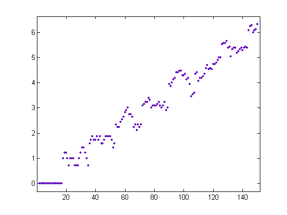
The values are arranged into "constellations" consisting of 18 elements each. A plot of √-½Σi=1xiM([x/i]) where M(1), M(2), M(3), ..., M(17) are set to 0 (along with bounding lines) for x=2, 3, 4, ..., 1000 is;
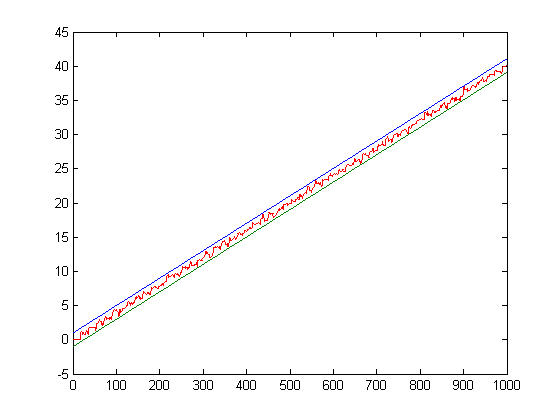
A plot of √-½Σi=1xiM([x/i]) where M(1), M(2), M(3), ..., M(40) are set to 0 for x=2, 3, 4, ..., 1000 is;
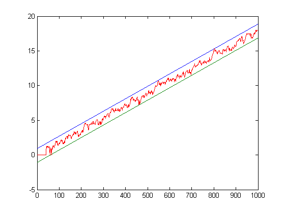
For a linear least-squares fit of the above values, the slope is 0.01795 and the intercept is -0.08879. As for other upper bounds of M values, the values appear to be bounded by parallel lines having intercepts equal to the intercept of the least-squares fit plus 1 and the intercept of the least-squares fit minus 1.
A quadratic least-squares fit of the slopes of the linear least-squares fits of √-½Σi=1xiM([x/i]) where the M values up to 3, 4, 5, ..., 10 are set to zero and for x=2, 3, 4, ..., 900 is;
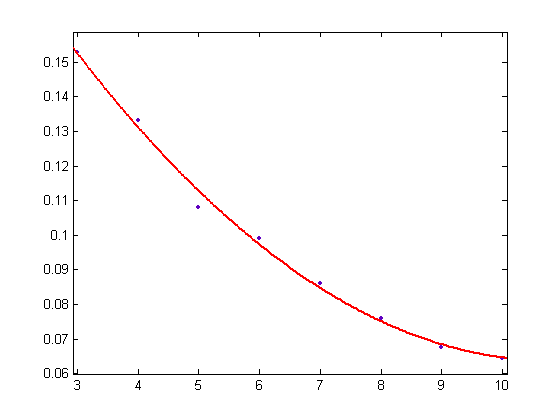
p1=0.001465 with a 95% confidence interval of (0.0009517, 0.001978), p2=-0.02575 with a 95% confidence interval of (-0.03048, -0.02102), and p3=0.1769 with a 95% confidence interval of (0.1676, 0.1862). SSE=3.346e-5, R-square=0.9952, adjusted R-square=0.9933, and RMSE=0.002587. For a linear least-squares fit of √-½Σi=2xiM([x/i]) for x=2, 3, 4, ..., 900, p1=0.153 with a 95% confidence interval of (0.1529, 0.153) and p2=0.004792 with a 95% confidence interval of (-0.01959, 0.02918). SSE=30.97, R-square=1, adjusted R-square=1, and RMSE=0.1858. The slope is not much different than that for √-½Σi=1xiM([x/i]) since M(x) is relatively small compared to Σi=2xiM([x/i]. Let y denote the minimum of x and 35. A plot of √-½Σi=1yiM([x/i]) for x=2, 3, 4, ..., 5128 is;
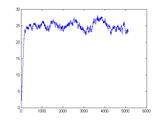
The values resemble a swept-frequency cosine signal. A program where M value lower bounds can be set is test1bb.
For a linear least-squares fit of √-½Σi=1xiM([x/i]) where only M(1) is set to 0 for x=2, 3, 4, ..., 900, p1=0.1885 with a 95% confidence interval of (0.1884, 0.1885) and p2=0.08875 with a 95% confidence interval of (0.07119, 0.1063). SSE=16.05, R-square=1, adjusted R-square=1, and RMSE=0.1063. A plot of √-½Σi=1xiM([x/i]) for x=2, 3, 4, ..., 101 is;
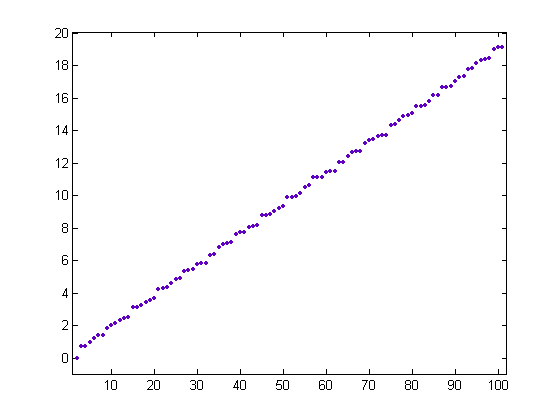
The values for x=4, 8, 16, 32, 64, ... equal the preceding values, otherwise the values increase monotonically. The values appear to be bounded by parallel lines having intercepts equal to the intercept of the least-squares fit plus 0.5 and the intercept of the least-squares fit minus 0.5. For a linear least-squares fit of √½Σi=1xiM([x/i]) where neither M(1) or M(3) is set to 0 for x=2, 3, 4, ..., 900, p1=0.3898 with a 95% confidence interval of (0.3898, 0.3899) and p2=0.1961 with a 95% confidence interval of (0.1842, 0.2079). SSE=7.279, R-square=1, adjusted R-square=1, and RMSE=0.09008. The values appear to increase monotonically and be bounded by parallel lines having intercepts equal to the intercept of the least-squares fit plus 0.25 and the intercept of the least-squares fit minus 0.25.
Let εv denote 2v/A(x)-rv for v=1, 2, 3, ..., A(x)/2. A plot of √Σv=1A(x)/2|εv| and √√(A(x)/2)Σv=1A(x)/2εv2 for x=3, 4, 5, ..., 2560 is;
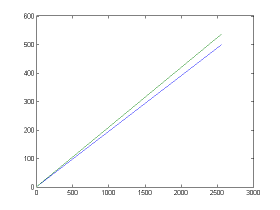
(√Σv=1A(x)/2|εv| is less than or equal to √√(A(x)/2)Σv=1A(x)/2εv2.) A plot of √√Σv=1A(x)/2|εv| and √A(x)Σv=1A(x)δv2 for x=3, 4, 5, ..., 2560 is;
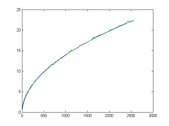
A program for computing these measures is test4fa. A subroutine used is merten4b. A program for computing the Mertens function up to x=5128 is test1bc. Subroutines used are haros5, uplolim, and mertens6. Another program for computing measures is test1b3a. A program for computing measures up to x=5128 is test4h. A subroutine used is merten4d.
A sequence xn of real numbers is uniformly distributed (mod 1) if and only if for every Riemann-integrable function f on [0, 1] one has limN→∞(1/N)Σn≤N f({xn})=∫10f(x)dx. (The brackets "{ }" denote the fractional part of the operand.) Some re-ordering of the sequence of square roots of the lengths of the sides of the polygon generated by a Farey sequence (probably corresponding to the lexicographic ordering used for the Farey fractions) appears to be uniformly distributed (mod 1). (See the section "Farey Points" in Kuipers and Niederreiter's Uniform Distribution of Sequences.) A program for confirming this for a few functions is test6f. (Multiple-word arithmetic is not used, so the results are not very accurate.)
A plot of (1/N)Σn≤N cos({xn}) for Farey sequences of orders 2, 3, 4, ..., 900 (where xn is the sequence of square roots of the lengths of the sides of the polygon) is;
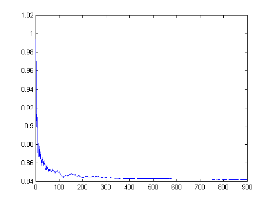
The expected value is sin(1) (0.84147). A program for generating these values is test1e. This program uses the subroutine haros1 to generate a Farey sequence. A plot of (1/N)Σn≤N{xn}2 for Farey sequences of orders 2, 3, 4, ..., 900 is;
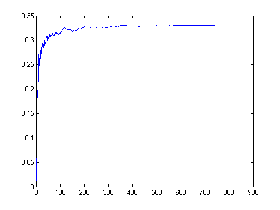
The expected value is 1/3.
Mém. Acad. Berlin, 23, année 1767, 1769, 7; Oeuvres, 2, 1868, 386-8.
Franel, J., and Landau, E.
Les suites de Farey et le problème des nombres premiers. Göttinger Nachr., 198-206 (1924).
Ramanujan, Srinivasa (1997)
Highly composite numbers, annotated by Jean-Louis Nicolas and Guy Robin, The Ramanujan Journal, 1:(2), 119-153
Robin, Guy (1984)
Grandes valeurs de la fonction somme des diviseurs et hypothèse de Riemann, Journal de Mathématiques Pures et Appliquées, Neuvième Série 63(2); 187-213
Lagarias, Jeffrey C. (2002)
An elementary problem equivalent to the Riemann hypothesis, The American Mathematical Monthly 109 (6):534-543
F. Mertens
Über eine zahlentheoretische Funktion, Akademie Wissenschaftlicher Wien Mathematik-Naturlich kleine Sitzungsber, 106 (1897) 761-830
P. Bachmann
Analytische Zahlentheorie, 402
Haselgrove, C. B. (1958)
"A disproof of a conjecture of Pólya". Mathematika 5: 141-145
Kuznetsov, E. (2011)
"Computing the Mertens function on a GPU", arXiv:1108:0135v1 [math.NT]
Software
Readers may copy and modify the above software. No guarantee is made that it is error-free.
A convolution of the differences of the zeta function zeros with the Möbius function is discussed at zeros. Associated software is at test3 (convolution with Möbius function), mobius, nucheck, primed, table2, test5c (compute probit function), test9a (compute Mertens function), test2n (Dirichlet products and Möbius inversion), interp1, test2g (Fourier transform of modified Riemann spectrum), zero1 (100,000 zeta function zeros), newrat3 (compute Riemann's R(x)), and nugauss (corresponding computations for Gaussian primes). The table of the first 10,000,000 zeta function zeros ("zerob.h") is not included. A 64-bit OS is required to run "test3". A summary of results pertaining to bounds of the Mertens function is given at bounds. Statistical properties of the zeta function zeros and standard uniform distributions are compared at unizeta. A general summary of this article is given at latest. Previous summaries (partially outdated) are at nuriem, newreim, and farreim. Let A(x) denote Σi=1xφ(i) where φ is Euler's totient function and let M(x) denote the Mertens function. A plot of √Σi=1xM([x/i])2, A(x)/√(x(x+1)(2x+1)/6), and |M(x)| versus √x for x=2, 3, 4, ..., 100000 is;

Σi=1xM([x/i])i=A(x) and by the Schwarz inequality A(x)/√(x(x+1)(2x+1)/6) is less than or equal to √Σi=1xM([x/i])2. (The brackets "[ ]" denote the floor function.) A plot of √Σi=1xM([x/i])2 versus √x for x=2, 3, 4, ..., 1000000 is;

A plot of Σi=1xM([x/i])2 and 8Σi=1xsgn(M([x/i]))-20 versus x for x=2, 3, 4, ..., 300 is;

(Note that Σi=1xsgn(M([x/i]))=O(x).) A plot of √Σi=1xM([x/i])2 and √8.7√Σi=1xsgn(M([x/i]))-2 versus x for x=2, 3, 4, ..., 1000 is;

Let k=[x/6] and r=x-6k. Let g(1), g(2), g(3), g(4), and g(5) equal 1, 2, 4, 6, and 11 respectively. If k>0 and r=0, let g(x)=12k+23(k(k-1))/2. If k>0 and r=1, let g(x)=12k+23(k(k-1))/2+7+6(k-1). If k>0 and r=2, let g(x)=12k+23(k(k-1))/2+11+9(k-1). If k>0 and r=3, let g(x)=12k+23(k(k-1))/2+17+13(k-1). If k>0 and r=4, let g(x)=12k+23(k(k-1))/2+22+16(k-1). If k>0 and r=5, let g(x)=12k+23(k(k-1))/2+33+22(k-1). g(x) is an empirically derived lower bound of Σi=1xsgn(M([x/i]))i. A plot of √Σi=1xsgn(M([x/i]))i-√g(x) versus x for x=2, 3, 4, ..., 200 is;

For a linear least-squares fit of √Σi=1xsgn(M([x/i]))i-√g(x) versus x for x=2, 3, 4, ..., 100000, p1=6.103e-5 with a 95% confidence interval of (6.103e-5, 6.104e-5), p2=3.05e-5 with a 95% confidence interval of (-0.0001669, 0.0002279), SSE=25.35, R-square=0.9999, and RMSE=0.01592. A plot with bounding lines having y-intercepts of 0.15 more and 0.15 less and the same slope is;

For a linear least-squares fit where x=2, 3, 4, ..., 1000000, p1=6.103e-5 with a 95% confidence interval of (6.103e-5, 6.103e-5), p2=-0.00046 with a 95% confidence interval of (-0.0005797, -0.0003404), SSE=931.5, R-square=1, and RMSE=0.03052. A plot with bounding lines having y-intercepts of 0.8 more and 0.8 less and the same slope is;

The variation in the √Σi=1xsgn(M([x/i]))i-√g(x) values appears to be slowly increasing. Based on this data, g(x)/√(x(x+1)(2x+1)/6) is a lower bound of √Σi=1x(sgn(M([x/i])))2. (Note that √Σi=1x(sgn(M([x/i])))2=O(x½).) Σi=1xsgn(M([x/i]))i is slightly greater than A(x). For a linear least-squares fit of √Σi=1xM([x/i])i versus x for x=2, 3, 4, ..., 50000, p1=0.5513 with a 95% confidence interval of (0.5513, 0.5513), p2=0.2758 with a 95% confidence interval of (0.2736, 0.2781), SSE=816.9, R-square=1, and RMSE=0.1278. For a linear least-squares fit of √Σi=1xM([x/i])1/3i versus x for x=2, 3, 4, ..., 50000, p1=0.5617 with a 95% confidence interval of (0.5617, 0.5617), p2=0.2809 with a 95% confidence interval of (0.2786, 0.2832), SSE=859, R-square=1, and RMSE=0.1311. For a linear least-squares fit of √Σi=1xM([x/i])1/5i versus x for x=2, 3, 4, ..., 50000, p1=0.5633 with a 95% confidence interval of (0.5633, 0.5633), p2=0.2817 with a 95% confidence interval of (0.2793, 0.284), SSE=890.9, R-square=1, and RMSE=0.1335. For a linear least-squares fit of √Σi=1xM([x/i])1/7i versus x for x=2, 3, 4, ..., 50000, p1=0.5639 with a 95% confidence interval of (0.5639, 0.5639), p2=0.282 with a 95% confidence interval of (0.2796, 0.2843), SSE=905.1, R-square=1, and RMSE=0.1345. For a linear least-squares fit of √Σi=1x sgn(M([x/i]))i versus x for x=2, 3, 4, ..., 50000, p1=0.5653 with a 95% confidence interval of (0.5653, 0.5653), p2=0.2827 with a 95% confidence interval of (0.2803, 0.2851), SSE=942.3, R-square=1, and RMSE=0.1373.
Let d denote the height of a step of the function √Σi=1xsgn(M([x/i]))i. d is less than or equal to 1.0. A histogram of [200d+0.5] for x≤500000 is;

(Two of the expected six step sizes are approximately equal.) Let e denote the height of a step of the function g(x). The bin-by-bin difference in the histograms of [200d+0.5] and [200e+0.5] for x≤1000000 is;

Let d denote the height of a step of the function √Σi=1xM([x/i])i. A histogram of [200d+0.5] for x≤500000 is;

Let d denote the height of a step of the function √Σi=1xM([x/i])1/3i. A histogram of [200d+0.5] for x≤500000 is;

Let h(x) denote Σi=1x(n[x/i]-m[x/i]) where mx denotes the number of fractions before 1/4 and nx denotes the number of fractions between 1/4 and 1/2 in a Farey sequence of order x. (Although 1/4<1/3<1/2, n3 is set to 0 since 1/4 is not in a Farey sequence of order 3.) h(2), h(3), h(4), ..., and h(13) equal 0, 0, 1, 1, 0, 1, 2, 1, 1, 2, 2, and 2 respectively and h(x+12)=h(x)+2 (based on empirical evidence). (The property Σi=1x(m[x/i]-n[x/i]+1/6)=1, 2/3, 1/2, 1/3, 1/6, 0, -1/6, -1/3, or -2/3 is analogous to the property Σi=1xM([x/i])=1 and can be proved similarly. As will be shown, there are infinitely many "Riemann hypotheses" associated with Farey sequences.) 12(h(x))2 is approximately equal to g(x) (for x>270, 12(h(x))2>g(x)). A plot of 12(h(x))2 and g(x) versus x for x=2, 3, 4, ..., 10000 is;

h(x) appears to be a lower bound of Σi=1xsgn(M([x/i])). A plot of Σi=1xsgn(M([x/i]))-h(x) versus x for x=2, 3, 4, ..., 1000 is;

Σi=1xsgn(M([x/i])) equals h(x) in 47 instances. A plot of h(x)-Σi=1xsgn(n[x/i]-m[x/i]) versus x for x=2, 3, 4, ..., 1000 is;

h(x) equals Σi=1xsgn(n[x/i]-m[x/i]) in 56 instances. A plot of Σi=1x(n[x/i]-m[x/i])2-Σi=1xsgn(M([x/i])) versus x for x=2, 3, 4, ..., 300 is;

1+Σi=1x(n[x/i]-m[x/i])2 equals Σi=1xsgn(M([x/i])) in 39 instances. Based on empirical evidence, log(x!)≥Σi=1xM([x/i])2≥ψ(x)≥Σi=1x|sgn(M([x/i]))|≥1+Σi=1x(n[x/i]-m[x/i])2 ≥Σi=1xsgn(M([x/i]))≥h(x)≥Σi=1xsgn(n[x/i]-m[x/i]). ψ(x) denotes the second Chebyshev function. Mertens proved that Σi=1xM([x/i])log(i)=ψ(x). Apparently, the log(i) factor is not large enough to give an upper bound of Σi=1xM([x/i])2. Σi=1xM([x/i])log(i)d(i)=log(x!) where d(i) denotes half the number of positive divisors of i. log(x!)=xlog(x)-x+O(log(x)), so this is a likely upper bound of Σi=1xM([x/i])2. (Since log(x) increases more slowly than any positive power of x, this is a better upper bound than x1+ε where ε>0.) A plot of log(x!), Σi=1xM([x/i])2, ψ(x), and Σi=1x|sgn(M([x/i]))| versus x for x=2, 3, 4, ..., 5000 is;

Σi=1xM([x/i])d(i)=x/2. d(i) is half the sum of positive divisors function σ0(i). (Σn=1∞σ0(n)/ns =ζ(s)2 where ζ(s) is the Riemann zeta function.) A plot of Σi=1x(n[x/i]-m[x/i])d(i) versus x for x=2, 3, 4, ..., 10250 is;

For a quadratic least-squares fit of Σi=1x(n[x/i]-m[x/i])d(i) versus x for x=2, 3, 4, ..., 10250, p1=1.016e-5 with a 95% confidence interval of (1.011e-5, 1.021e-5), p2=0.5924 with a 95% confidence interval of (0.5918, 0.5929), p3=-106.6 with a 95% confidence interval of (-107.8, -105.4), SSE=4.373e+6, R-square=0.9999, and RMSE=20.66. A plot of log(x!)/12-Σi=1x(n[x/i]-m[x/i])d(i) versus x for x=2, 3, 4, ..., 40000 is;

A plot of 5Σi=1x(m[x/i]-n[x/i]+1/6 )σ0(i) versus x for x=2, 3, 4, ..., 5000 is;

For a linear least-squares fit of 5Σi=1x(m[x/i]-n[x/i]+1/6)σ0(i) versus x for x=2, 3, 4, ..., 5000, p1=0.999 with a 95% confidence interval of (0.9985, 0.9994), p2=0.003815 with a 95% confidence interval of (-1.233, 1.24), SSE=2.481e+6, R-square=0.9998, and RMSE=22.28. For a linear least-squares fit of 5Σi=1x(m[x/i]-n[x/i]+1/6)σ0(i) versus x for x=2, 3, 4, ..., 40000, p1=0.9989 with a 95% confidence interval of (0.9989, 0.9989), p2=0.136 with a 95% confidence interval of (-0.6118, 0.88381), SSE=5.821e+7, R-square=1, and RMSE=38.15.
Σi=1xM([x/i])σ1(i)=x(x+1)/2. A plot of x(x+1)/24 and Σi=1x(n[x/i]-m[x/i])σ1(i) versus x for x=2, 3, 4, ..., 10250 is;

For a quadratic least-squares fit of Σi=1x(n[x/i]-m[x/i])σ1(i) versus x for x=2, 3, 4, ..., 10250, p1=0.03945 with a 95% confidence interval of (0.03945, 0.03946), p2=-0.04567 with a 95% confidence interval of (-0.06933, -0.02201), p3=2.278 with a 95% confidence interval of (-50.24, 54.8), SSE=8.366e+9, R-square=1, and RMSE=903.6. For a quadratic least-squares fit of Σi=1x(n[x/i]-m[x/i])σ1(i) versus x for x=2, 3, 4, ..., 40000, p1=0.03945 with a 95% confidence interval of (0.03945, 0.03945), p2=-0.04398 with a 95% confidence interval of (-0.05599, -0.03197), p3=0.4941 with a 95% confidence interval of (-103.5, 104.5), SSE=5.004e+11, R-square=1, and RMSE=3537. A plot of x(x+1)/2 and 5.13Σi=1x(m[x/i]-n[x/i]+1/6)σ1(i) versus x for x=2, 3, 4, ..., 100 is;

Σi=1xM([x/i])σ2(i)=x(x+1)(2x+1)/6. A plot of x(x+1)(2x+1)/6 and 5.36Σi=1x(m[x/i]-n[x/i]+1/6)σ2(i) versus x for x=2, 3, 4, ..., 200 is;

Ramanujan proved that the Riemann hypothesis implies σ1(n)<eγnlog(log(n)) for sufficiently large n where γ denotes Euler's constant. (Robin proved that this inequality is true for all n≥5041 if and only if the Riemann hypothesis is true.) A plot of M(x)+eγΣi=2xM([x/i])ilog(log(i)), 12((nx-mx)+eγΣi=2x(n[x/i]-m[x/i])ilog(log(i))), and x(x+1)/2 versus x for x=2, 3, 4, ..., 200 is;

A plot of M(x)+eγΣi=2xM([x/i])ilog(log(i))-5.14((mx-nx+1/6)+eγΣi=2x(m[x/i]-n[x/i]+1/6)ilog(log(i))) versus x for x=2, 3, 4, ..., 1000 is;

A plot of M(x)+eγΣi=2xM([x/i])ilog(log(i)), eγA(x), and x(x+1)/2 versus x for x=2, 3, 4, ..., 200 is;

eγA(x)>x(x+1)/2, eγΣi=1xsgn(M([x/i]))i>Σi=1xsgn(M([x/i]))σ1(i), and eγΣi=1x|sgn(M([x/i]))|i>Σi=1x|sgn(M([x/i]))|σ1(i). (These inequalities are related to Bachmann's theorem that σ(1)+σ(2)+...+σ(n)=(1/12)π2n2+O(nlog n)). A plot of |M(x)|+eγΣi=2x|M([x/i])|ilog(log(i)), Σi=1x|M([x/i])|σ1(i), 12(|nx-mx|+eγΣi=2x|n[x/i]-m[x/i]|ilog(log(i))), and A(x) versus x for x=2, 3, 4, ..., 200 is;

A plot of sgn(M(x))+eγΣi=2xsgn(M([x/i]))ilog(log(i)), 12(sgn(nx-mx)+eγΣi=2xsgn(n[x/i]-m[x/i])ilog(log(i))), and Σi=1xsgn(M([x/i]))σ1(i), versus x for x=2, 3, 4, ..., 200 is;

2+eγA(x)>Σi=1xsgn(M([x/i]))σ1(i). (Upper bounds of partial sums of Σi=1xsgn(M([x/i]))σ1(i) are determined in the following.) A plot of M(x)+eγΣi=2xM([x/i])ilog(log(i)), 12((nx-mx)+eγΣi=2x(n[x/i]-m[x/i])ilog(log(i))), and x(x+1)/2 versus x for x=2, 3, 4, ..., 10250 is;

For a quadratic least-squares fit of M(x)+eγΣi=2xM([x/i])ilog(log(i)) versus x for x=2, 3, 4, ..., 10250, p1=1.253 with a 95% confidence interval of (1.253, 1.253), p2=-485.3 with a 95% confidence interval of (-487.5, -483.1), p3=2.93e+5 with a 95% confidence interval of (2.881e+5, 2.979e+5), SSE=7.322e+13, R-square=1, and RMSE=8.453e+4. For a quadratic least-squares fit of 12((nx-mx)+eγΣi=2x(n[x/i]-m[x/i])ilog(log(i))) versus x for x=2, 3, 4, ..., 10250, p1=1.081 with a 95% confidence interval of (1.081, 1.081), p2=-587.5 with a 95% confidence interval of (-590.2, -584.8), p3=3.46e+5 with a 95% confidence interval of (3.401e+5, 3.519e+5), SSE=1.061e+14, R-square=1, and RMSE=1.018e+5. Let Hn=Σj=1n1/j. Lagarias proved that Σd|nd≤Hn+exp(Hn)log(Hn) (with equality only for n=1) if and only if the Riemann hypothesis is true. A plot of Σi=1xM([x/i])(Hn+exp(Hn)log(Hn)), 12Σi=1x(n[x/i]-m[x/i])(Hn+exp(Hn)log(Hn)), and x(x+1)/2 versus x=2, 3, 4, ..., 200 is;

A plot of Σi=1xM([x/i])(Hn+exp(Hn)log(Hn)) and 5.134Σi=1x(m[x/i]-n[x/i]+1/6)(Hn+exp(Hn)log(Hn)) (superimposed on each other) versus x for x=2, 3, 4, ..., 5000 is;

A plot of Σi=1xM([x/i])(Hn+exp(Hn)log(Hn))-5.134Σi=1x(m[x/i]-n[x/i]+1/6)(Hn+exp(Hn)log(Hn)) versus x for x=2, 3, 4, ..., 5000 is;

A plot of Σi=1xd(i)-xlog(x)/2 versus x for x=2, 3, 4, ..., 3000 is;

A plot of log(x!), Σi=1xlog(i)/d(i), and Σi=1xM([x/i])2 versus x for x=2, 3, 4, ..., 2000 is;

A plot of ψ(x) and Σi=1x(n[x/i]-m[x/i])log(i) versus x for x=2, 3, 4, ..., 10250 is;

ψ(x) is the more linear of the two curves. For a quadratic least-squares fit of Σi=1x(n[x/i]-m[x/i])log(i) versus x for x=2, 3, 4, ..., 10250, p1=2.006e-5 with a 95% confidence interval of (1.995e-5, 2.017e-5), p2=0.9945 with a 95% confidence interval of (0.9933, 0.9957), p3=-215.9 with a 95% confidence interval of (-218.5, -213.2), SSE=2.103e+7, R-square=0.9998, and RMSE=45.3. A plot of log(x!)-6Σi=1x(n[x/i]-m[x/i])log(i) versus x for x=2, 3, 4, ..., 40000 is;

For a linear least-squares fit of log(x!)-6Σi=1x(n[x/i]-m[x/i])log(i) versus x for x=2, 3, 4, ..., 40000, p1=1.201 with a 95% confidence interval of (1.201, 1.201), p2=-31.92 with a 95% confidence interval of (-35.4, -28.44), SSE=1.262e+9, R-square=0.9998, and RMSE=177.6. A plot of 5Σi=1x(m[x/i]-n[x/i]+1/6)log(i) versus x for x=2, 3, 4, ..., 5000 is;

For a linear least-squares fit of 5Σi=1x(m[x/i]-n[x/i]+1/6)log(i) versus x for x=2, 3, 4, ..., 5000, p1=0.9959 with a 95% confidence interval of (0.9949, 0.997), p2=4.395 with a 95% confidence interval of (1.411, 7.379), SSE=1.445e+7, R-square=0.9986, and RMSE=53.78. For a linear least-squares fit of 5Σi=1x(m[x/i]-n[x/i]+1/6)log(i) versus x for x=2, 3, 4, ..., 40000, p1=1.001 with a 95% confidence interval of (1.001, 1.001), p2=-26.6 with a 95% confidence interval of (-29.5, -23.7), SSE=8.765e+8, R-square=0.9998, and RMSE=148.
A plot of log(x!) and Σi=1x(n[x/i]-m[x/i])log(i)d(i) versus x for x=2, 3, 4, ..., 10250 is;

A plot of log(x!)-Σi=1x(n[x/i]-m[x/i])log(i)d(i) versus x for x=2, 3, 4, ..., 10250 is;

For a quadratic least-squares fit of log(x!)-Σi=1x(n[x/i]-m[x/i])log(i)d(i) versus x for x=2, 3, 4, ..., 10250, p1=-3.112e-5 with a 95% confidence interval of (-3.118e-5, -3.106e-5), p2=3.684 with a 95% confidence interval of (3.684, 3.685), p3=-97.64 with a 95% confidence interval of (-99.09, -96.19), SSE=6.402e+6, R-square=1, and RMSE=25. For a quadratic least-squares fit of log(x!)-Σi=1x(n[x/i]-m[x/i])log(i)d(i) versus x for x=2, 3, 4, ..., 40000, p1=-1.506e-5 with a 95% confidence interval of (-1.508e-5, -1.504e-5), p2=3.409 with a 95% confidence interval of (3.409, 3.41), p3=746.4 with a 95% confidence interval of (738.8, 753.9), SSE=2.655e+9, R-square=0.9999, and RMSE=257.6. A plot of 5Σi=1x(m[x/i]-n[x/i]+1/6)log(i)d(i) and log(x!) (superimposed on each other) versus x for x=2, 3, 4, ..., 40000 is;

A plot of log(x!)-4.99Σi=1x(m[x/i]-n[x/i]+1/6)log(i)d(i) versus x for x=2, 3, 4, ..., 40000 is;

A plot of log(x!), Σi=1x(n[x/i]-m[x/i])log(i)d(i), and Σi=1xM([x/i])2 versus x for x=2, 3, 4, ..., 1000 is;

Also, 2/3≥(1/x)Σi=1x|sgn(M([x/i]))|-(1/x)Σi=1xsgn(M([x/i])). Also, Σi=1xsgn(M([x/i])) is approximately equal to Σi=1x|sgn(n[x/i]-m[x/i])| (for x≤5128, 16≥|Σi=1xsgn(M([x/i]))-Σi=1x|sgn(n[x/i]-m[x/i])|) and Σi=1x|sgn(n[x/i]-m[x/i])|≥Σi=1xsgn(n[x/i]-m[x/i]). A plot of Σi=1xsgn(M([x/i])) and Σi=1x|sgn(n[x/i]-m[x/i])|-20 versus x for x=2, 3, 4, ..., 5128 is;

For a linear least-squares fit of Σi=1xsgn(M([x/i])) versus x for x=2, 3, 4, ..., 10250, p1=0.1739 with a 95% confidence interval of (0.1739, 0.1739), p2=0.1087 with a 95% confidence interval of (0.004574, 0.2128), SSE=7.402e+4, R-square=1, and RMSE=2.688. For a linear least-squares fit of Σi=1x|sgn(n[x/i]-m[x/i])| versus x for x=2, 3, 4, ..., 10250, p1=0.1727 with a 95% confidence interval of (0.1727, 0.1727), p2=-0.4368 with a 95% confidence interval of (-0.5234, -0.3502), SSE=5.122e+4, R-square=1, and RMSE=2.236. A plot of √Σi=1xsgn(M([x/i]))-√Σi=1x|sgn(n[x/i]-m[x/i])| versus x for x=2, 3, 4, ..., 5128 is;

A plot of (1/x)Σi=1xsgn(M([x/i]))-(1/x)Σi=1x|sgn(n[x/i]-m[x/i])| versus x for x=2, 3, 4, ..., 170 is;

The arc beginning with the value 0.5 consists of terms from the harmonic sequence. Another arc consists of the terms -1/22, -1/44, -1/57, -1/60, -1/88, -1/112, -1/123, -1/125, -1/133, -1/134, -1/135, -1/137, -1/144, -1/153, .... Another arc consists of the terms -2/114, -2/124, -2/136, .... Another arc consists of the terms 2/19, 2/31, 2/43, 2/47, 2/63, 2/73, 2/74, 2/75, 2/86, 2/87, 2/95, 2/97, 2/98, 2/102, 2/103, 2/107, 2/109, 2/117, 2/126, 2/127, 2/130, 2/139, 2/146, 2/147, 2/151, 2/161, ... Another arc consists of the terms 3/65, 3/100, 3/101, 3/163, .... Another arc consists of the terms 4/99, 4/131, 4/162, .... For x in the vicinity of 10250, (1/x)Σi=1xsgn(M([x/i]))-(1/x)Σi=1x|sgn(n[x/i]-m[x/i])| is less than 0.0025.
A plot of (1/x)Σi=1xsgn(M([x/i]))-(1/x)Σi=1x|sgn(n[x/i]-m[x/i])| versus x for x=49000, 49001, 49002,..., 50000 is;

If x>56, g(x)>12Σi=1x(n[x/i]-m[x/i])i and if x>78, (h(x))2>Σi=1x(n[x/i]-m[x/i])i. Also, Σi=1x(n[x/i]-m[x/i])i≥Σi=1xsgn(n[x/i]-m[x/i])i. In general, mx-nx corresponds to M(x). A "Riemann hypothesis" for the Farey sequence is that nx-mx=O(x½).
The following two plots show the correspondence between mx-nx and M(x). A plot of M(x) for x=2, 3, 4, ..., 5128 is;

A plot of mx-nx for x=2, 3, 4, ..., 5128 is;

Constraints on the growth of |mx-nx| are determined by the density of the primes. In the following, lower and upper bounds of mx (and nx) are determined. Denote the lower bound by L(x) and the upper bound by U(x). U(x)-L(x)=3+Σ[logq(x)]+Σ[logq(x/2)] where the summation is over the primes q of the form 4k+3 that are less than or equal to x. A plot of 1.5x/log(x)-(U(x)-L(x)) versus x for x=2, 3, 4, ..., 50000 is;

For a quadratic least-squares fit of 1.5x/log(x)-(U(x)-L(x)) versus x for x=2, 3, 4, ..., 50000, p1=-9.077e-8 with a 95% confidence interval of (-9.104e-8, -9.05e-8), p2=0.06182 with a 95% confidence interval of (0.06181, 0.06184), p3=10.07 with a 95% confidence interval of (9.92, 10.23), SSE=1.689e+6, R-square=1, and RMSE=5.812. For a quadratic least-squares fit of 1.5x/log(x)-(U(x)-L(x)) versus x for x=2, 3, 4, ..., 100000, p1=-4.287e-8 with a 95% confidence interval of (-4.295e-8, -4.279e-8), p2=0.05926 with a 95% confidence interval of (0.05925, 0.05927), p3=32.53 with a 95% confidence interval of (32.34, 32.71), SSE=9.426e+6, R-square=1, and RMSE=9.709. A plot of 1.5x/log(x) and U(x)-L(x) versus x for x=2, 3, 4, ..., 200 is;

A plot of √(U(x)-L(x)) and |nx-mx| versus x for x=2, 3, 4, ..., 50000 is;

A histogram of the mx-nx values for x=2, 3, 4, ..., 10000 superimposed on a normal probability distribution having the same mean and standard deviation (-0.9805 and 12.6148 respectively) is;

Let s(x) denote the standard deviation of the distribution of mi-ni values from i=2 to x. A plot of 3+2.4s(x) and √(U(x)-L(x)) versus x for x=2, 3, 4, ..., 20000 is;

A plot of s(x) and 0.385√(x/log(x)) versus x for x=2, 3, 4, ..., 50000 is;

Let ox denote the number of fractions less than 1/5 and px the number of fractions greater than 1/5 and less than 2/5 in a Farey sequence of order x. A plot of upper and lower bounds of ox (computed by determining whether 5 divides φ(n)) and ox for x=2, 3, 4, ..., 200 is;

A plot of the square root of the corresponding upper bound minus the corresponding lower bound and |ox-px| for x=2, 3, 4, ..., 12000 is;

Let qx denote the number of fractions less than 1/6 and rx the number of fractions greater than 1/6 and less than 1/3 in a Farey sequence of order x. A plot of the square root of the corresponding upper bound minus the corresponding lower bound and |qx-rx| for x=2, 3, 4, ..., 12000 is;

Let s(x) denote the standard deviation of the distribution of qi-ri values from i=2 to x. A plot of 5.2s(x) and the square roots of the upper bounds minus the lower bounds for x=2, 3, 4, ..., 10000 is;

Let sx denote the number of fractions less than 1/7 and tx the number of fractions greater than 1/7 and less than 2/7 in a Farey sequence of order x. A plot of the square root of the corresponding upper bound minus the corresponding lower bound and |sx-tx| for x=2, 3, 4, ..., 12000 is;

Let ux denote the number of fractions less than 1/8 and vx the number of fractions greater than 1/8 and less than 1/4 in a Farey sequence of order x. A plot of the standard deviations of the distributions of mi-ni, qi-ri, and ui-vi values from i=2 to x and (1/8.4)√x versus x for x=2, 3, 4, ..., 50000 is;

Let h5(x) denote Σi=1x(p[x/i]-o[x/i]), let h6(x) denote Σi=1x(r[x/i]-q[x/i]), let h7(x) denote Σi=1x(t[x/i]-s[x/i]), and let h8(x) denote Σi=1x(v[x/i]-u[x/i]). Based on empirical evidence, h5(x+5)=h5(x)+2, h6(x+6)=h6(x)+2, h7(x+7)=h7(x)+3, and h8(x+8)=h8(x)+3. (p3 and p4 are set to 1 and 2 respectively, r4 and r5 are set to 1 and 2 respectively, t4, t5, and t6 are set to 1, 2, and 3 respectively, and v5, v6, and v7 are set to 1, 2, and 3 respectively. If n3 is set to 1 instead of 0, then h(x+4)=h(x)+1.) These slopes determine the factors required to "linearize" Σi=1x(p[x/i]-o[x/i])log(i), Σi=1x(r[x/i]-q[x/i])log(i), Σi=1x(t[x/i]-s[x/i])log(i), and Σi=1x(v[x/i]-u[x/i])log(i). As previously shown, the factor required for Σi=1x(n[x/i]-m[x/i])log(i) is 12/2. A plot of log(x!)-(5/2)Σi=1x(p[x/i]-o[x/i])log(i) versus x for x=2, 3, 4, ..., 10000 is;

A plot of log(x!)-(6/2)Σi=1x(r[x/i]-q[x/i])log(i) versus x for x=2, 3, 4, ..., 10000 is;

A plot of log(x!)-(7/3)Σi=1x(t[x/i]-s[x/i])log(i) versus x for x=2, 3, 4, ..., 10000 is;

A plot of (2/5)log(x!)-Σi=1x(p[x/i]-o[x/i])σ0(i) versus x for x=2, 3, 4, ..., 10000 is;

A plot of (2/6)log(x!)-Σi=1x(r[x/i]-q[x/i])σ0(i) versus x for x=2, 3, 4, ..., 10000 is;

A plot of (3/7)log(x!)-Σi=1x(t[x/i]-s[x/i])σ0(i) versus x for x=2, 3, 4, ..., 10000 is;

For a quadratic least-squares fit of log(x!)-(2/5)Σi=1x(p[x/i]-o[x/i])log(i)d(i) versus x for x=2, 3, 4, ..., 10000, p1=-3.041e-5 with a 95% confidence interval of (-3.045e-5, -3.037e-5), p2=3.553 with a 95% confidence interval of (3.553, 3.553), p3=-93.21 with a 95% confidence interval of (-94.15, -92.27), SSE=2.549e+6, R-square=1, and RMSE=15.97. For a quadratic least-squares fit of log(x!)-(1/2)Σi=1x(r[x/i]-q[x/i])log(i)d(i) versus x for x=2, 3, 4, ..., 10000, p1=-2.999e-5 with a 95% confidence interval of (-3.003e-5, -2.995e-5), p2=3.763 with a 95% confidence interval of (3.762, 3.763), p3=-113.8 with a 95% confidence interval of (-114.7, -112.9), SSE=2.437e+6, R-square=1, and RMSE=15.61. For a quadratic least-squares fit of log(x!)-(3/7)Σi=1x(t[x/i]-s[x/i])log(i)d(i) versus x for x=2, 3, 4, ..., 10000, p1=-4.499e-5 with a 95% confidence interval of (-4.507e-5, -4.491e-5), p2=3.464 with a 95% confidence interval of (3.463, 3.465), p3=-6.292 with a 95% confidence interval of (-8.189, -4.394), SSE=1.039e+7, R-square=1, and RMSE=32.25.
A plot of log(x!)-2.3679Σi=1x(q[x/i]-r[x/i]+1/3)log(i)d(i) versus x for x=2, 3, 4, ..., 40000 is;

For a linear least-squares fit of 2.3725Σi=1x(q[x/i]-r[x/i]+1/3)σ0(i) versus x for x=2, 3, 4, ..., 40000, p1=1 with a 95% confidence interval of (1, 1), p2=0.1345 with a 95% confidence interval of (-0.08722, 0.3563), SSE=5.118e+6, R-square=1, and RMSE=11.31. For a linear least-squares fit of 2.3730Σi=1x(q[x/i]-r[x/i]+1/3)log(i) versus x for x=2, 3, 4, ..., 40000, p1=1 with a 95% confidence interval of (0.9999, 1), p2=2.909 with a 95% confidence interval of (1.367, 4.451), SSE=2.476e+8, R-square=1, and RMSE=78.67.
A plot of log(x!)-1.793Σi=1x(s[x/i]-t[x/i]+3/7)log(i)d(i) versus x for x=2, 3, 4, ..., 40000 is;

For a linear least-squares fit of 1.795Σi=1x(s[x/i]-t[x/i]+3/7)σ0(i) versus x for x=2, 3, 4, ..., 40000, p1=1 with a 95% confidence interval of (1, 1), p2=0.1419 with a 95% confidence interval of (-0.04282, 0.3266), SSE=3.551e+6, R-square=1, and RMSE=9.422. For a linear least-squares fit of 1.794Σi=1x(s[x/i]-t[x/i]+3/7)log(i) versus x for x=2, 3, 4, ..., 40000, p1=0.9999 with a 95% confidence interval of (0.9999, 0.9999), p2=-6.001 with a 95% confidence interval of (-7.125, -4.878), SSE=1.313e+8, R-square=1, and RMSE=57.3.
Let yx(n) denote the number of fractions less than 1/n and zx(n) the number of fractions greater than 1/n and less than 2/n in a Farey sequence of order x. A plot of the p1 values of the linear least-squares fits of Σi=1x(y[x/i](n)-z[x/i](n)+[(n-1)/2]/n)σ0(i) versus x for x=2, 3, 4, ..., 4000 and n=4, 5, 6, ..., 15 is;

A quadratic least-squares fit of the p1 values of the linear least-squares fits of Σi=1x(y[x/i](n)-z[x/i](n)+[(n-1)/2]/n)σ0(i) versus x for x=2, 3, 4, ..., 4000 and n=4, 6, 8, ..., 14 is;

A quadratic least-squares fit of the p1 values of the linear least-squares fits of Σi=1x(y[x/i](n)-z[x/i](n)+[(n-1)/2]/n)σ0(i) versus x for x=2, 3, 4, ..., 4000 and n=5, 7, 9, ..., 15 is;

A plot of the p1 and p2 values of the quadratic least-squares fits of Σi=1x(y[x/i](n)-z[x/i](n)+[(n-1)/2]/n)σ1(i) versus x for x=2, 3, 4, ..., 4000 and n=4, 5, 6, ..., 15 is;

A quartic least-squares fit of the p1 values of the quadratic least-squares fits of Σi=1x(y[x/i](n)-z[x/i](n)+[(n-1)/2]/n)σ1(i) versus x for x=2, 3, 4, ..., 4000 and n=4, 6, 8, ..., 14 is;

A quartic least-squares fit of the p1 values of the quadratic least-squares fits of Σi=1x(y[x/i](n)-z[x/i](n)+[(n-1)/2]/n)σ1(i) versus x for x=2, 3, 4, ..., 4000 and n=5, 7, 9, ..., 15 is;

A sixth-order polynomial least-squares fit of the p1 values of the cubic least-squares fits of Σi=1x(y[x/i](n)-z[x/i](n)+[(n-1)/2]/n)σ2(i) versus x for x=2, 3, 4, ..., 2000 and n=5, 7, 9, ..., 31 is;

A plot of yx(65)-zx(65) versus x for x=2, 3, 4, ..., 1625 is;

A plot of yx(200)-zx(200) versus x for x=2, 3, 4, ..., 5000 is;

A plot of yx(200)-zx(200) versus x for x=100, 200, 300, 400, ..., 5000 is;

For even n, the limits of (yn/2(n)-zn/2(n))/n, (yn(n)-zn(n))/n, (y3n/2(n)-z3n/2(n))/n, (y2n(n)-z2n(n))/n,..., as n approaches infinity appear to be -1/2, -1/4, -1/3, -1/6, -2/5, -2/15, -31/105, -29/140, -19/42, -41/420, -76/385, -201/1540, -751/1430, -1109/4004, -803/2718, -857/13411, -3577/11807, -721/17163, -738/2897, ..., respectively. Superimposed plots of (y2(4)-z2(4))/4, (y4(4)-z4(4))/4, (y6(4)-z6(4))/4, ..., (y200(4)-z200(4))/4 and (y500000(1000000)-z500000(1000000))/1000000, (y1000000(1000000)-z1000000(1000000))/1000000, (y1500000(1000000)-z1500000(1000000))/1000000, ..., (y50000000(1000000)-z50000000(1000000))/1000000 are;

Let δm(x), m=1, 2, 3, ..., denote the interpolated normalized difference in the number of fractions in a Farey sequence computed using the above limits (m-1 values between successive limits are interpolated). A cubic least-squares fit of -Σi=1xδ4([x/i])σ2(i) versus x for x=2, 3, 4, ..., 76 is;

These values were computed using 19 limits. A quadratic least-squares fit of -Σi=1xδ4([x/i])σ1(i) versus x for x=2, 3, 4, ..., 76 is;

A linear least-squares fit of Σi=1xδ4([x/i])2 versus x for x=2, 3, 4, ..., 76 is;

A plot of (1/12)xlog(x), -Σi=1xδ4([x/i])log(i), and -Σi=1xδ4([x/i]) versus x for x=2, 3, 4, ... 76 is;

When a small number of limits is considered, there appears to be less "noise" in the curve of Σi=1xδ1([x/i])2 values than in the curve of Σi=1xδ1([x/i]) values. A superimposed plot of the SSE values of the linear least-squares fits of Σi=1xδ1([x/i]), Σi=1xδ2([x/i]), Σi=1xδ3([x/i]), ..., Σi=1xδ8([x/i]) for x=400, 800, 1200, ..., 3200 respectively and the SSE values of the linear least-squares fits of Σi=1xδ1([x/i])2, Σi=1xδ2([x/i])2, Σi=1xδ3([x/i])2, ..., Σi=1xδ8([x/i])2 for x=400, 800, 1200, ..., 3200 respectively is;

These values were computed using 400 approximate limits (accurate to about 6 decimal places). A superimposed plot of the RMSE values of the linear least-squares fits of Σi=1xδ1([x/i]), Σi=1xδ2([x/i]), Σi=1xδ3([x/i]), ..., Σi=1xδ8([x/i]) for x=400, 800, 1200, ..., 3200 respectively and the RMSE values of the linear least-squares fits of Σi=1xδ1([x/i])2, Σi=1xδ2([x/i])2, Σi=1xδ3([x/i])2, ..., Σi=1xδ8([x/i])2 for x=400, 800, 1200, ..., 3200 respectively is;

A plot of 6.6666Σi=1x(δ1([x/i])+0.1704)M(i) and Σi=1xM([x/i])M(i) versus x for x=2, 3, 4, ... 999 is;

These values were computed using 1000 approximate limits. The slope of the curve of -Σi=1xδ1([x/i]) values for x=2, 3, 4, ..., 999 (as given by a linear least-squares fit) is about 0.1704.
Let L(i) denote the summatory Liouville function. A plot of √Σi=1xM([x/i])L(i)2 and √Σi=1x(δ1([x/i])+0.1704)L(i)2 versus x for x=2, 3, 4, ... 999 is;

Let Λ denote the Mangoldt function. A plot of -Σi=1xδ1([x/i]) and -Σi=1xδ1([x/i])Λ(i) for x=2, 3, 4, ..., 999 is;

For a linear least-squares fit of -Σi=1xδ1([x/i]) versus x for x=2, 3, 4, ..., 999, p1=0.1704 with a 95% confidence interval of (0.1703, 0.1706), p2=-0.04484 with a 95% confidence interval of (-0.1291, 0.03936), SSE=455.6, R-square=0.9998, and RMSE=0.6763. For a linear least-squares fit of -Σi=1xδ1([x/i])Λ(i) versus x for x=2, 3, 4, ..., 999, p1=0.17 with a 95% confidence interval of (0.1695, 0.1705), p2=-0.2796 with a 95% confidence interval of (-0.5688, 0.009683), SSE=5374, R-square=0.9978, and RMSE=2.323. A plot of the p1 values of the linear least-squares fits of -Σi=1xδ1([x/i])Λ(i), -Σi=1xδ2([x/i])Λ(i), -Σi=1xδ3([x/i])Λ(i), ..., -Σi=1xδ36([x/i])Λ(i) versus x for x up to 999, 1999, 2999, ..., 35999 respectively is;

For a linear least-squares fit of -Σi=1xδ100([x/i]) versus x for x=2, 3, 4, ..., 99999, p1=0.01936 with a 95% confidence interval of (0.01936, 0.01936), p2=-0.1094 with a 95% confidence interval of (-0.1154, -0.1034), SSE=2.347e+4, R-square=1, and RMSE=0.4845. For a linear least-squares fit of -Σi=1xδ100([x/i])Λ(i) versus x for x=2, 3, 4, ..., 99999, p1=0.01936 with a 95% confidence interval of (0.01936, 0.01936), p2=-0.6391 with a 95% confidence interval of (-0.6584, -0.6198), SSE=2.415e+5, R-square=1, and RMSE=1.554. A plot of -Σi=1xδ100([x/i]) and -Σi=1xδ100([x/i])Λ(i) (superimposed on each other) for x=2, 3, 4, ..., 99999 is;

A plot of -Σi=1xδ1([x/i]) and -Σi=1xδ1([x/i])Λ(i) (where the approximate limits are accurate to about 3 decimal places) for x=2, 3, 4, ..., 9999 is;

Σi=1xM([x/i])Λ(i)=-Σi=1xμ(i)log(i) where μ(i) is the Möbius function. (Σi=1xμ(i)log(i) is usually denoted by H(x). H(x)/(xlog(x))→0 as x→∞ and limx→∞(M(x)/x-H(x)/(xlog(x)))=0.) A plot of Σi=1x(z[x/i](4)-y[x/i](4))Λ(i), -Σi=1xδ1([x/i])Λ(i), and Σi=1xM([x/i])Λ(i) for x=2, 3, 4, ..., 9999 is;

Σi=1x(y[x/i](4)-z[x/i](4)+1/4)Λ(i) is approximately equal to Σi=1xM([x/i])Λ(i). A plot of (1/(xlog(x)))Σi=1x(δ1([x/i])+0.1704)Λ(i) for x=2, 3, 4, ..., 9999 is;

A plot of Λ*Λ (the Dirichlet product of Λ with itself) for x=2, 3, 4, ..., 999 is;

Let (α◦F)(x) denote Σn≤xα(n)F([x/n]) where α is an arithmetical function. (Usually, (α◦F)(x) denotes Σn≤xα(n)F(x/n) where F is a real or complex-valued function defined on (0, +∞) such that F(x)=0 for 0<x<1.) As expected, Λ◦(Λ◦δ1)=(Λ*Λ)◦δ1. Let u(n)=1 for all n. A quadratic least squares fit of (u◦δ1)◦δ1 (where the limits are accurate to about 6 decimal places) for x=2, 3, 4, ..., 999 is;

p1=0.008421 with a 95% confidence interval of (0.008414, 0.008428), p2=0.001703 with a 95% confidence interval of (-0.005279, 0.008684), p3=-0.01665 with a 95% confidence interval of (-1.53, 1.497), SSE=6.483e+4, R-square=1, and RMSE=8.072. A quadratic least-squares fit of (Λ◦δ1)◦δ1 for x=2, 3, 4, ..., 999 is;

p1=0.00847 with a 95% confidence interval of (0.008459, 0.008428), p2=-0.09465 with a 95% confidence interval of (-0.1054, -0.08391), p3=4.914 with a 95% confidence interval of (2.586, 7.242), SSE=1.534e+5, R-square=1, and RMSE=12.42. For a quadratic least-squares fit of -(Λ◦δ1)◦Λ for x=2, 3, 4, ..., 999, p1=0.01802 with a 95% confidence interval of (0.01798, 0.01806), p2=-0.3354 with a 95% confidence interval of (-0.3761, -0.2946), p3=22.13 with a 95% confidence interval of (13.3, 30.97), SSE=2.208e+6 R-square=0.9999, and RMSE=47.1. Λ◦(Λ◦δ1) and δ1◦(Λ◦δ1) appear to be O(xlog(x)). A plot of -Λ◦(Λ◦δ1) for x=2, 3, 4, ..., 999 is;

Let dx(n) denote (yx(n)-zx(n))/n. A quadratic least-squares fit of (Λ◦d(4))◦d(4) versus x for x=2, 3, 4, ..., 2000 is;

A cubic least-squares fit of -((Λ◦d(4))◦d(4))◦d(4) versus x for x=2, 3, 4, ..., 5000 is;

Let ck(n) denote Ramanujan's sum. A plot of ∑i=1x(ck([x/i])+1)(yi(n)-zi(n)) for k=17, n=50, and x=2, 3, 4, ..., 1500 is;

A plot of Σi=1x(n[x/i]-m[x/i])M(i) versus x for x=2, 3, 4, ..., 5000 is;

A plot of Σi=1x(m[x/i]-n[x/i]+1/6)M(i) versus x for x=2, 3, 4, ..., 5000 is;

A plot of Σi=1xM([x/i])M(i) versus x for x=2, 3, 4, ..., 4000000 is;

A plot of log(x!) (computed using Stieltjes' approximation) and |Σi=1xM([x/i])M(i)| versus x for x=2, 3, 4, ..., 100000 is;

The oscillations of Σi=1xM([x/i])M(i) appear to be due to the first non-trivial zero of the zeta function. (Haselgrove used Ingham's smoothing function to disprove the Pólya conjecture and gives the corresponding smoothing function for the Merten's conjecture.) A plot of x(log(x))2 and |Σi=1xM([x/i])M(i)| versus x for x=2, 3, 4, ..., 2000000 is;

A plot of Σi=1xM([x/i])2 and Σi=1x(m[x/i]-n[x/i]+1/6)M([x/i]) versus x for x=2, 3, 4, ..., 5000 is;

(43/30)+Σi=1x(m[x/i]-n[x/i]+1/6)M([x/i])≥(1/5)Σi=1xM([x/i])2. (11/300)+Σi=1x(m[x/i]-n[x/i]+1/6)2≥(1/25)Σi=1xM([x/i])2.
A plot of Σi=1xm[x/i]M(i) versus x for x=2, 3, 4, ..., 5000 is;

For a quadratic least-squares fit of Σi=1xm[x/i]M(i) versus x for x=2, 3, 4, ..., 5000, p1=0.03205 with a 95% confidence interval of (0.03205, 0.03205), p2=1.317 with a 95% confidence interval of (1.297, 1.337), p3=-29.2 with a 95% confidence interval of (-50.44, -7.957), SSE=3.25e+8, R-square=1, and RMSE=255.1.
Based on empirical evidence, ([x/n]([x/n]+1))/2≥-Σi=1[x/(j+1)]sgn(M([x/i]))i≥0, j=1, 2, 3, ..., where n=2+Σi=1j|sgn(M(i))|. A plot of ([x/n]([x/n]+1))/2+Σi=1[x/(j+1)]sgn(M([x/i]))i for j=1 and x=2, 3, 4, ..., 1000 is;

([x/n]([x/n]+1))/2 equals -Σi=1[x/(j+1)]sgn(M([x/i]))i in 194 instances. Let k=Σi=1j|sgn(M(i))| and let r=(k-1)-[(k-1)/4]4. Let d=2, 3, 3, or 4 when r=0, 1, 2, or 3 respectively. Based on empirical evidence, 1+([x/n]([x/n]+1))/2≥-Σi=1[x/(j+1)]sgn(M([x/i]))σ1(i)≥0, j=1, 2, 3, ..., where n=3[(k-1)/4]+d. A plot of 1+([x/n]([x/n]+1))/2+Σi=1[x/(j+1)]sgn(M([x/i]))σ1(i) for j=3 and x=2, 3, 4, ..., 200 is;

A plot of (1/x)Σi=1[x/10]σ1(i) versus x for x=2, 3, 4, ..., 200 is;

A plot of -(1/x)Σi=1[x/10]sgn(M([x/i]))σ1(i) versus x for x=2, 3, 4, ..., 200 is;

A plot of (1/x)Σi=1[x/10]|sgn(M([x/i]))|σ1(i) versus x for x=2, 3, 4, ..., 200 is;

A plot of (1/x)Σi=1[x/40]σ1(i)-(1/x)Σi=1[x/40]|sgn(M([x/i]))|σ1(i) versus x for x=2, 3, 4, ..., 300 is;

The bottom arc of values corresponds to x values where M(x)=0. A plot of (1/x)Σi=1[x/100]σ1(i)-(1/x)Σi=1[x/100]|sgn(M([x/i]))|σ1(i) versus x for x=2, 3, 4, ..., 500 is;

A plot of (1/x)Σi=1[x/200]σ1(i)-(1/x)Σi=1[x/200]|sgn(M([x/i]))|σ1(i) versus x for x=2, 3, 4, ..., 2000 is;

A table of the x, M(x), (1/x)Σi=1[x/200]σ1(i)-(1/x)Σi=1[x/200]|sgn(M([x/i]))|σ1(i) (denoted by "delta sums"), (1/x)Σi=1[x/200]σ1(i) (denoted by "sigma sum"), and (1/x)Σi=1[x/200]σ1(i)/((1/x)Σi=1[x/200]σ1(i)-(1/x)Σi=1[x/200]|sgn(M([x/i]))|σ1(i)) (denoted by "ratio") values associated with the different arcs is;
  x  M(x)  delta sums	 sigma sum	ratio
		  arc #1
 214   0 4.672897e-003 4.672897e-003 1.000000e+000
 231   0 4.329004e-003 4.329004e-003 1.000000e+000
 232   0 4.310345e-003 4.310345e-003 1.000000e+000
 235   0 4.255319e-003 4.255319e-003 1.000000e+000
 236   0 4.237288e-003 4.237288e-003 1.000000e+000
 238   0 4.201681e-003 4.201681e-003 1.000000e+000
 254   0 3.937008e-003 3.937008e-003 1.000000e+000
 329   0 3.039514e-003 3.039514e-003 1.000000e+000
 331   0 3.021148e-003 3.021148e-003 1.000000e+000
 332   0 3.012048e-003 3.012048e-003 1.000000e+000
 333   0 3.003003e-003 3.003003e-003 1.000000e+000
 353   0 2.832861e-003 2.832861e-003 1.000000e+000
 355   0 2.816901e-003 2.816901e-003 1.000000e+000
 356   0 2.808989e-003 2.808989e-003 1.000000e+000
 358   0 2.793296e-003 2.793296e-003 1.000000e+000
 362   0 2.762431e-003 2.762431e-003 1.000000e+000
 363   0 2.754821e-003 2.754821e-003 1.000000e+000
 364   0 2.747253e-003 2.747253e-003 1.000000e+000
 366   0 2.732240e-003 2.732240e-003 1.000000e+000
 393   0 2.544529e-003 2.544529e-003 1.000000e+000
 401   0 2.493766e-003 9.975062e-003 4.000000e+000
 403   0 2.481390e-003 9.925558e-003 4.000000e+000
 404   0 2.475248e-003 9.900990e-003 4.000000e+000
 405   0 2.469136e-003 9.876543e-003 4.000000e+000
 407   0 2.457002e-003 9.828010e-003 4.000000e+000
 408   0 2.450980e-003 9.803922e-003 4.000000e+000
 413   0 2.421308e-003 9.685230e-003 4.000000e+000
 414   0 2.415459e-003 9.661836e-003 4.000000e+000
 419   0 2.386635e-003 9.546539e-003 4.000000e+000
 420   0 2.380952e-003 9.523810e-003 4.000000e+000
 422   0 2.369668e-003 9.478673e-003 4.000000e+000
 423   0 2.364066e-003 9.456265e-003 4.000000e+000
 424   0 2.358491e-003 9.433962e-003 4.000000e+000
 425   0 2.352941e-003 9.411765e-003 4.000000e+000
 427   0 2.341920e-003 9.367681e-003 4.000000e+000
 537   0 1.862197e-003 7.448790e-003 4.000000e+000
 541   0 1.848429e-003 7.393715e-003 4.000000e+000
 607   0 1.647446e-003 1.317957e-002 8.000000e+000
 608   0 1.644737e-003 1.315789e-002 8.000000e+000
 635   0 1.574803e-003 1.259843e-002 8.000000e+000
 636   0 1.572327e-003 1.257862e-002 8.000000e+000
 637   0 1.569859e-003 1.255887e-002 8.000000e+000
 781   0 1.280410e-003 1.024328e-002 8.000000e+000
 785   0 1.273885e-003 1.019108e-002 8.000000e+000
 793   0 1.261034e-003 1.008827e-002 8.000000e+000
 795   0 1.257862e-003 1.006289e-002 8.000000e+000
 796   0 1.256281e-003 1.005025e-002 8.000000e+000
 798   0 1.253133e-003 1.002506e-002 8.000000e+000
 812   0 1.231527e-003 1.847291e-002 1.500000e+001
 823   0 1.215067e-003 1.822600e-002 1.500000e+001
 824   0 1.213592e-003 1.820388e-002 1.500000e+001
 825   0 1.212121e-003 1.818182e-002 1.500000e+001
 853   0 1.172333e-003 1.758499e-002 1.500000e+001
 869   0 1.150748e-003 1.726122e-002 1.500000e+001
 877   0 1.140251e-003 1.710376e-002 1.500000e+001
 883   0 1.132503e-003 1.698754e-002 1.500000e+001
 884   0 1.131222e-003 1.696833e-002 1.500000e+001
 886   0 1.128668e-003 1.693002e-002 1.500000e+001
 889   0 1.124859e-003 1.687289e-002 1.500000e+001
 893   0 1.119821e-003 1.679731e-002 1.500000e+001
 895   0 1.117318e-003 1.675978e-002 1.500000e+001
 896   0 1.116071e-003 1.674107e-002 1.500000e+001
 898   0 1.113586e-003 1.670379e-002 1.500000e+001
 903   0 1.107420e-003 1.661130e-002 1.500000e+001
 904   0 1.106195e-003 1.659292e-002 1.500000e+001
 906   0 1.103753e-003 1.655629e-002 1.500000e+001
 910   0 1.098901e-003 1.648352e-002 1.500000e+001
 913   0 1.095290e-003 1.642935e-002 1.500000e+001
 915   0 1.092896e-003 1.639344e-002 1.500000e+001
 916   0 1.091703e-003 1.637555e-002 1.500000e+001
 919   0 1.088139e-003 1.632209e-002 1.500000e+001
 920   0 1.086957e-003 1.630435e-002 1.500000e+001
 1002  0 9.980040e-004 2.095808e-002 2.100000e+001
 1005  0 9.950249e-004 2.089552e-002 2.100000e+001
 1010  0 9.900990e-004 2.079208e-002 2.100000e+001
 1013  0 9.871668e-004 2.073050e-002 2.100000e+001
 1014  0 9.861933e-004 2.071006e-002 2.100000e+001
 1219  0 8.203445e-004 2.707137e-002 3.300000e+001
 1220  0 8.196721e-004 2.704918e-002 3.300000e+001
 1255  0 7.968127e-004 2.629482e-002 3.300000e+001
 1256  0 7.961783e-004 2.627389e-002 3.300000e+001
 1279  0 7.818608e-004 2.580141e-002 3.300000e+001
 1280  0 7.812500e-004 2.578125e-002 3.300000e+001
 1291  0 7.745933e-004 2.556158e-002 3.300000e+001
 1292  0 7.739938e-004 2.554180e-002 3.300000e+001
 1297  0 7.710100e-004 2.544333e-002 3.300000e+001
 1299  0 7.698229e-004 2.540416e-002 3.300000e+001
 1300  0 7.692308e-004 2.538462e-002 3.300000e+001
 1302  0 7.680492e-004 2.534562e-002 3.300000e+001
 1306  0 7.656968e-004 2.526799e-002 3.300000e+001
 1336  0 7.485030e-004 2.470060e-002 3.300000e+001
 1338  0 7.473842e-004 2.466368e-002 3.300000e+001
 1342  0 7.451565e-004 2.459016e-002 3.300000e+001
 1491  0 6.706908e-004 2.749832e-002 4.100000e+001
 1492  0 6.702413e-004 2.747989e-002 4.100000e+001
 1518  0 6.587615e-004 2.700922e-002 4.100000e+001
 1519  0 6.583278e-004 2.699144e-002 4.100000e+001
 1520  0 6.578947e-004 2.697368e-002 4.100000e+001
 1521  0 6.574622e-004 2.695595e-002 4.100000e+001
 1523  0 6.565988e-004 2.692055e-002 4.100000e+001
 1531  0 6.531679e-004 2.677988e-002 4.100000e+001
 1532  0 6.527415e-004 2.676240e-002 4.100000e+001
 1537  0 6.506181e-004 2.667534e-002 4.100000e+001
 1543  0 6.480881e-004 2.657161e-002 4.100000e+001
 1544  0 6.476684e-004 2.655440e-002 4.100000e+001
 1546  0 6.468305e-004 2.652005e-002 4.100000e+001
 1843  0 5.425936e-004 3.743896e-002 6.900000e+001
 1844  0 5.422993e-004 3.741866e-002 6.900000e+001
 1845  0 5.420054e-004 3.739837e-002 6.900000e+001
 1864  0 5.364807e-004 3.701717e-002 6.900000e+001
 1866  0 5.359057e-004 3.697749e-002 6.900000e+001
 1938  0 5.159959e-004 3.560372e-002 6.900000e+001

		  arc #2
 429   -1 6.993007e-003 9.324009e-003 1.333333e+000
 462   -5 6.493506e-003 8.658009e-003 1.333333e+000
 463   -6 6.479482e-003 8.639309e-003 1.333333e+000
 464   -6 6.465517e-003 8.620690e-003 1.333333e+000
 465   -7 6.451613e-003 8.602151e-003 1.333333e+000
 470   -7 6.382979e-003 8.510638e-003 1.333333e+000
 471   -6 6.369427e-003 8.492569e-003 1.333333e+000
 472   -6 6.355932e-003 8.474576e-003 1.333333e+000
 473   -5 6.342495e-003 8.456660e-003 1.333333e+000
 476   -6 6.302521e-003 8.403361e-003 1.333333e+000
 477   -6 6.289308e-003 8.385744e-003 1.333333e+000
 508   -5 5.905512e-003 7.874016e-003 1.333333e+000
 509   -6 5.893910e-003 7.858546e-003 1.333333e+000
 658   -9 4.559271e-003 1.215805e-002 2.666667e+000
 659  -10 4.552352e-003 1.213961e-002 2.666667e+000
 662  -10 4.531722e-003 1.208459e-002 2.666667e+000
 663  -11 4.524887e-003 1.206637e-002 2.666667e+000
 664  -11 4.518072e-003 1.204819e-002 2.666667e+000
 665  -12 4.511278e-003 1.203008e-002 2.666667e+000
 666  -12 4.504505e-003 1.201201e-002 2.666667e+000
 667  -11 4.497751e-003 1.199400e-002 2.666667e+000
 711   -5 4.219409e-003 1.125176e-002 2.666667e+000
 712   -5 4.213483e-003 1.123596e-002 2.666667e+000
 713   -4 4.207574e-003 1.122020e-002 2.666667e+000
 717   -3 4.184100e-003 1.115760e-002 2.666667e+000
 724   -1 4.143646e-003 1.104972e-002 2.666667e+000
 725   -1 4.137931e-003 1.103448e-002 2.666667e+000
 726   -1 4.132231e-003 1.101928e-002 2.666667e+000
 727   -2 4.126547e-003 1.100413e-002 2.666667e+000
 728   -2 4.120879e-003 1.098901e-002 2.666667e+000
 729   -2 4.115226e-003 1.097394e-002 2.666667e+000
 732   -2 4.098361e-003 1.092896e-002 2.666667e+000
 733   -3 4.092769e-003 1.091405e-002 2.666667e+000
 786   -1 3.816794e-003 1.017812e-002 2.666667e+000
 787   -2 3.811944e-003 1.016518e-002 2.666667e+000
 802	2 3.740648e-003 1.870324e-002 5.000000e+000
 803	3 3.735990e-003 1.867995e-002 5.000000e+000
 806	1 3.722084e-003 1.861042e-002 5.000000e+000
 807	2 3.717472e-003 1.858736e-002 5.000000e+000
 808	2 3.712871e-003 1.856436e-002 5.000000e+000
 809	1 3.708282e-003 1.854141e-002 5.000000e+000
 810	1 3.703704e-003 1.851852e-002 5.000000e+000
 815	1 3.680982e-003 1.840491e-002 5.000000e+000
 816	1 3.676471e-003 1.838235e-002 5.000000e+000
 817	2 3.671971e-003 1.835985e-002 5.000000e+000
 826   -1 3.631961e-003 1.815981e-002 5.000000e+000
 827   -2 3.627570e-003 1.813785e-002 5.000000e+000
 828   -2 3.623188e-003 1.811594e-002 5.000000e+000
 829   -3 3.618818e-003 1.809409e-002 5.000000e+000
 838   -2 3.579952e-003 1.789976e-002 5.000000e+000
 839   -3 3.575685e-003 1.787843e-002 5.000000e+000
 840   -3 3.571429e-003 1.785714e-002 5.000000e+000
 841   -3 3.567182e-003 1.783591e-002 5.000000e+000
 844   -1 3.554502e-003 1.777251e-002 5.000000e+000
 845   -1 3.550296e-003 1.775148e-002 5.000000e+000
 846   -1 3.546099e-003 1.773050e-002 5.000000e+000
 847   -1 3.541913e-003 1.770956e-002 5.000000e+000
 848   -1 3.537736e-003 1.768868e-002 5.000000e+000
 851	1 3.525264e-003 1.762632e-002 5.000000e+000
 854   -1 3.512881e-003 1.756440e-002 5.000000e+000
 855   -1 3.508772e-003 1.754386e-002 5.000000e+000
 1082  -5 2.772643e-003 1.940850e-002 7.000000e+000
 1083  -5 2.770083e-003 1.939058e-002 7.000000e+000
 1562  -4 1.920615e-003 2.624840e-002 1.366667e+001
 1563  -3 1.919386e-003 2.623161e-002 1.366667e+001
 1570  -3 1.910828e-003 2.611465e-002 1.366667e+001
 1571  -4 1.909612e-003 2.609803e-002 1.366667e+001
 1586  -7 1.891551e-003 2.585120e-002 1.366667e+001
 1587  -7 1.890359e-003 2.583491e-002 1.366667e+001
 1590  -5 1.886792e-003 2.578616e-002 1.366667e+001
 1591  -4 1.885607e-003 2.576996e-002 1.366667e+001
 1592  -4 1.884422e-003 2.575377e-002 1.366667e+001
 1593  -4 1.883239e-003 2.573760e-002 1.366667e+001
 1596  -4 1.879699e-003 2.568922e-002 1.366667e+001
 1597  -5 1.878522e-003 2.567314e-002 1.366667e+001
 1706 -13 1.758499e-003 3.282532e-002 1.866667e+001
 1707 -12 1.757469e-003 3.280609e-002 1.866667e+001
 1738  -9 1.726122e-003 3.222094e-002 1.866667e+001
 1739  -8 1.725129e-003 3.220242e-002 1.866667e+001
 1754 -11 1.710376e-003 3.192702e-002 1.866667e+001
 1755 -11 1.709402e-003 3.190883e-002 1.866667e+001
 1786  -7 1.679731e-003 3.135498e-002 1.866667e+001
 1787  -8 1.678791e-003 3.133744e-002 1.866667e+001
 1772  -7 1.693002e-003 3.160271e-002 1.866667e+001
 1773  -7 1.692047e-003 3.158488e-002 1.866667e+001
 1796  -7 1.670379e-003 3.118040e-002 1.866667e+001
 1797  -6 1.669449e-003 3.116305e-002 1.866667e+001
 1806  -6 1.661130e-003 3.820598e-002 2.300000e+001
 1807  -5 1.660210e-003 3.818484e-002 2.300000e+001
 1808  -5 1.659292e-003 3.816372e-002 2.300000e+001
 1809  -5 1.658375e-003 3.814262e-002 2.300000e+001
 1827  -4 1.642036e-003 3.776683e-002 2.300000e+001
 1838  -2 1.632209e-003 3.754081e-002 2.300000e+001
 1839  -1 1.631321e-003 3.752039e-002 2.300000e+001
 1840  -1 1.630435e-003 3.750000e-002 2.300000e+001

		  arc #3
 428	0 9.345794e-003 9.345794e-003 1.000000e+000
 642   -3 6.230530e-003 1.246106e-002 2.000000e+000
 643   -4 6.220840e-003 1.244168e-002 2.000000e+000
 644   -4 6.211180e-003 1.242236e-002 2.000000e+000
 693   -9 5.772006e-003 1.154401e-002 2.000000e+000
 694   -8 5.763689e-003 1.152738e-002 2.000000e+000
 695   -7 5.755396e-003 1.151079e-002 2.000000e+000
 696   -7 5.747126e-003 1.149425e-002 2.000000e+000
 697   -6 5.738881e-003 1.147776e-002 2.000000e+000
 698   -5 5.730659e-003 1.146132e-002 2.000000e+000
 705   -5 5.673759e-003 1.134752e-002 2.000000e+000
 708   -3 5.649718e-003 1.129944e-002 2.000000e+000
 709   -4 5.641749e-003 1.128350e-002 2.000000e+000
 714   -3 5.602241e-003 1.120448e-002 2.000000e+000
 715   -4 5.594406e-003 1.118881e-002 2.000000e+000
 762   -5 5.249344e-003 1.049869e-002 2.000000e+000
 763   -4 5.242464e-003 1.048493e-002 2.000000e+000
 764   -4 5.235602e-003 1.047120e-002 2.000000e+000
 811	0 4.932182e-003 1.849568e-002 3.750000e+000
 814	0 4.914005e-003 1.842752e-002 3.750000e+000
 849	0 4.711425e-003 1.766784e-002 3.750000e+000
 850	0 4.705882e-003 1.764706e-002 3.750000e+000
 987	1 4.052685e-003 1.519757e-002 3.750000e+000
 988	1 4.048583e-003 1.518219e-002 3.750000e+000
 989	2 4.044489e-003 1.516684e-002 3.750000e+000
 993	2 4.028197e-003 1.510574e-002 3.750000e+000
 994	1 4.024145e-003 1.509054e-002 3.750000e+000
 995	2 4.020101e-003 1.507538e-002 3.750000e+000
 996	2 4.016064e-003 1.506024e-002 3.750000e+000
 997	1 4.012036e-003 1.504514e-002 3.750000e+000
 998	2 4.008016e-003 1.503006e-002 3.750000e+000
 999	2 4.004004e-003 1.501502e-002 3.750000e+000
 1000	2 4.000000e-003 2.100000e-002 5.250000e+000
 1001	1 3.996004e-003 2.097902e-002 5.250000e+000
 1059  -4 3.777148e-003 1.983003e-002 5.250000e+000
 1060  -4 3.773585e-003 1.981132e-002 5.250000e+000
 1061  -5 3.770028e-003 1.979265e-002 5.250000e+000
 1065  -7 3.755869e-003 1.971831e-002 5.250000e+000
 1066  -8 3.752345e-003 1.969981e-002 5.250000e+000
 1067  -7 3.748828e-003 1.968135e-002 5.250000e+000
 1068  -7 3.745318e-003 1.966292e-002 5.250000e+000
 1069  -8 3.741815e-003 1.964453e-002 5.250000e+000
 1076  -9 3.717472e-003 1.951673e-002 5.250000e+000
 1086  -7 3.683241e-003 1.933702e-002 5.250000e+000
 1087  -8 3.679853e-003 1.931923e-002 5.250000e+000
 1088  -8 3.676471e-003 1.930147e-002 5.250000e+000
 1089  -8 3.673095e-003 1.928375e-002 5.250000e+000
 1090  -9 3.669725e-003 1.926606e-002 5.250000e+000
 1091 -10 3.666361e-003 1.924840e-002 5.250000e+000
 1092 -10 3.663004e-003 1.923077e-002 5.250000e+000
 1093 -11 3.659652e-003 1.921317e-002 5.250000e+000
 1094 -10 3.656307e-003 1.919561e-002 5.250000e+000
 1098 -12 3.642987e-003 1.912568e-002 5.250000e+000
 1099 -11 3.639672e-003 1.910828e-002 5.250000e+000
 1100 -11 3.636364e-003 1.909091e-002 5.250000e+000
 1203  -3 3.325021e-003 2.743142e-002 8.250000e+000
 1204  -3 3.322259e-003 2.740864e-002 8.250000e+000
 1205  -2 3.319502e-003 2.738589e-002 8.250000e+000
 1209  -2 3.308519e-003 2.729529e-002 8.250000e+000
 1210  -2 3.305785e-003 2.727273e-002 8.250000e+000
 1211  -1 3.303055e-003 2.725021e-002 8.250000e+000
 1212  -1 3.300330e-003 2.722772e-002 8.250000e+000
 1213  -2 3.297609e-003 2.720528e-002 8.250000e+000
 1221  -1 3.276003e-003 2.702703e-002 8.250000e+000
 1222  -2 3.273322e-003 2.700491e-002 8.250000e+000
 1223  -3 3.270646e-003 2.698283e-002 8.250000e+000
 1224  -3 3.267974e-003 2.696078e-002 8.250000e+000
 1225  -3 3.265306e-003 2.693878e-002 8.250000e+000
 1226  -2 3.262643e-003 2.691680e-002 8.250000e+000
 1239  -3 3.228410e-003 2.663438e-002 8.250000e+000
 1240  -3 3.225806e-003 2.661290e-002 8.250000e+000
 1241  -2 3.223207e-003 2.659146e-002 8.250000e+000
 1242  -2 3.220612e-003 2.657005e-002 8.250000e+000
 1243  -1 3.218021e-003 2.654867e-002 8.250000e+000
 1244  -1 3.215434e-003 2.652733e-002 8.250000e+000
 1257	1 3.182180e-003 2.625298e-002 8.250000e+000
 1259  -1 3.177125e-003 2.621128e-002 8.250000e+000
 1260  -1 3.174603e-003 2.619048e-002 8.250000e+000
 1262	1 3.169572e-003 2.614897e-002 8.250000e+000
 1267	1 3.157064e-003 2.604578e-002 8.250000e+000
 1268	1 3.154574e-003 2.602524e-002 8.250000e+000
 1269	1 3.152088e-003 2.600473e-002 8.250000e+000
 1276	2 3.134796e-003 2.586207e-002 8.250000e+000
 1277	1 3.132341e-003 2.584182e-002 8.250000e+000
 1281  -1 3.122560e-003 2.576112e-002 8.250000e+000
 1283  -1 3.117693e-003 2.572097e-002 8.250000e+000
 1611 -10 2.482930e-003 3.476102e-002 1.400000e+001
 1825  -3 2.191781e-003 3.780822e-002 1.725000e+001
 1841	0 2.172732e-003 3.747963e-002 1.725000e+001
 1912  -5 2.092050e-003 3.608787e-002 1.725000e+001
 1913  -6 2.090957e-003 3.606900e-002 1.725000e+001

		    arc #4
 1258	0 3.974563e-003 2.623211e-002 6.600000e+000
 1261	0 3.965107e-003 2.616971e-002 6.600000e+000
 1266	0 3.949447e-003 2.606635e-002 6.600000e+000
 1282	0 3.900156e-003 2.574103e-002 6.600000e+000

		    arc #5
 1071  -9 5.602241e-003 1.960784e-002 3.500000e+000
 1072  -9 5.597015e-003 1.958955e-002 3.500000e+000
 1073  -8 5.591799e-003 1.957130e-002 3.500000e+000
 1155  -5 5.194805e-003 1.818182e-002 3.500000e+000
 1156  -5 5.190311e-003 1.816609e-002 3.500000e+000
 1157  -4 5.185825e-003 1.815039e-002 3.500000e+000
 1158  -5 5.181347e-003 1.813472e-002 3.500000e+000
 1159  -4 5.176877e-003 1.811907e-002 3.500000e+000
 1160  -4 5.172414e-003 1.810345e-002 3.500000e+000
 1161  -4 5.167959e-003 1.808786e-002 3.500000e+000
 1162  -5 5.163511e-003 1.807229e-002 3.500000e+000
 1163  -6 5.159071e-003 1.805675e-002 3.500000e+000
 1164  -6 5.154639e-003 1.804124e-002 3.500000e+000
 1175  -5 5.106383e-003 1.787234e-002 3.500000e+000
 1176  -5 5.102041e-003 1.785714e-002 3.500000e+000
 1177  -4 5.097706e-003 1.784197e-002 3.500000e+000
 1178  -5 5.093379e-003 1.782683e-002 3.500000e+000
 1182  -7 5.076142e-003 1.776650e-002 3.500000e+000
 1183  -7 5.071851e-003 1.775148e-002 3.500000e+000
 1184  -7 5.067568e-003 1.773649e-002 3.500000e+000
 1190  -6 5.042017e-003 1.764706e-002 3.500000e+000
 1191  -5 5.037783e-003 1.763224e-002 3.500000e+000
 1192  -5 5.033557e-003 1.761745e-002 3.500000e+000
 1193  -6 5.029338e-003 1.760268e-002 3.500000e+000
 1194  -7 5.025126e-003 1.758794e-002 3.500000e+000
 1660 -10 3.614458e-003 3.373494e-002 9.333333e+000
 1661  -9 3.612282e-003 3.371463e-002 9.333333e+000
 1662 -10 3.610108e-003 3.369434e-002 9.333333e+000
 1663 -11 3.607937e-003 3.367408e-002 9.333333e+000
 1664 -11 3.605769e-003 3.365385e-002 9.333333e+000
 1665 -11 3.603604e-003 3.363363e-002 9.333333e+000
 1765  -8 3.399433e-003 3.172805e-002 9.333333e+000
 1775  -6 3.380282e-003 3.154930e-002 9.333333e+000
 1776  -6 3.378378e-003 3.153153e-002 9.333333e+000
 1777  -7 3.376477e-003 3.151379e-002 9.333333e+000
 1794  -8 3.344482e-003 3.121516e-002 9.333333e+000
 1810  -6 3.314917e-003 3.812155e-002 1.150000e+001
 1811  -7 3.313087e-003 3.810050e-002 1.150000e+001
 1814  -6 3.307607e-003 3.803749e-002 1.150000e+001
 1815  -6 3.305785e-003 3.801653e-002 1.150000e+001
 1816  -6 3.303965e-003 3.799559e-002 1.150000e+001
 1817  -5 3.302146e-003 3.797468e-002 1.150000e+001
 1818  -5 3.300330e-003 3.795380e-002 1.150000e+001
 1819  -4 3.298516e-003 3.793293e-002 1.150000e+001
 1834  -5 3.271538e-003 3.762268e-002 1.150000e+001
 1965	3 3.053435e-003 3.511450e-002 1.150000e+001
 1966	4 3.051882e-003 3.509664e-002 1.150000e+001
 1967	5 3.050330e-003 3.507880e-002 1.150000e+001
 1968	5 3.048780e-003 3.506098e-002 1.150000e+001
 1969	6 3.047232e-003 3.504317e-002 1.150000e+001

		     arc #6
 706   -4 9.915014e-003 1.133144e-002 1.142857e+000
 707   -3 9.900990e-003 1.131542e-002 1.142857e+000
 710   -5 9.859155e-003 1.126761e-002 1.142857e+000
 716   -4 9.776536e-003 1.117318e-002 1.142857e+000
 858   -1 8.158508e-003 1.748252e-002 2.142857e+000
 859   -2 8.149010e-003 1.746217e-002 2.142857e+000
 924	3 7.575758e-003 1.623377e-002 2.142857e+000
 925	3 7.567568e-003 1.621622e-002 2.142857e+000
 926	4 7.559395e-003 1.619870e-002 2.142857e+000
 927	4 7.551241e-003 1.618123e-002 2.142857e+000
 928	4 7.543103e-003 1.616379e-002 2.142857e+000
 929	3 7.534984e-003 1.614639e-002 2.142857e+000
 930	4 7.526882e-003 1.612903e-002 2.142857e+000
 931	4 7.518797e-003 1.611171e-002 2.142857e+000
 940	4 7.446809e-003 1.595745e-002 2.142857e+000
 941	3 7.438895e-003 1.594049e-002 2.142857e+000
 942	2 7.430998e-003 1.592357e-002 2.142857e+000
 943	3 7.423118e-003 1.590668e-002 2.142857e+000
 944	3 7.415254e-003 1.588983e-002 2.142857e+000
 945	3 7.407407e-003 1.587302e-002 2.142857e+000
 946	2 7.399577e-003 1.585624e-002 2.142857e+000
 947	1 7.391763e-003 1.583949e-002 2.142857e+000
 952	3 7.352941e-003 1.575630e-002 2.142857e+000
 953	2 7.345226e-003 1.573977e-002 2.142857e+000
 954	2 7.337526e-003 1.572327e-002 2.142857e+000
 955	3 7.329843e-003 1.570681e-002 2.142857e+000
 1016  -1 6.889764e-003 2.066929e-002 3.000000e+000
 1017  -1 6.882989e-003 2.064897e-002 3.000000e+000
 1019  -1 6.869480e-003 2.060844e-002 3.000000e+000
 1075  -9 6.511628e-003 1.953488e-002 3.000000e+000
 1214  -1 5.766063e-003 2.718287e-002 4.714286e+000
 1215  -1 5.761317e-003 2.716049e-002 4.714286e+000
 1216  -1 5.756579e-003 2.713816e-002 4.714286e+000
 1217  -2 5.751849e-003 2.711586e-002 4.714286e+000
 1275	2 5.490196e-003 2.588235e-002 4.714286e+000
 1316  -2 5.319149e-003 2.507599e-002 4.714286e+000
 1317  -1 5.315110e-003 2.505695e-002 4.714286e+000
 1319  -1 5.307051e-003 2.501895e-002 4.714286e+000
 1324  -1 5.287009e-003 2.492447e-002 4.714286e+000
 1325  -1 5.283019e-003 2.490566e-002 4.714286e+000
 1327  -1 5.275057e-003 2.486812e-002 4.714286e+000
 1328  -1 5.271084e-003 2.484940e-002 4.714286e+000
 1330	1 5.263158e-003 2.481203e-002 4.714286e+000
 1331	1 5.259204e-003 2.479339e-002 4.714286e+000
 1332	1 5.255255e-003 2.477477e-002 4.714286e+000
 1333	2 5.251313e-003 2.475619e-002 4.714286e+000
 1334	1 5.247376e-003 2.473763e-002 4.714286e+000
 1422  12 4.922644e-003 2.883263e-002 5.857143e+000
 1423  11 4.919185e-003 2.881237e-002 5.857143e+000
 1424  11 4.915730e-003 2.879213e-002 5.857143e+000
 1425  11 4.912281e-003 2.877193e-002 5.857143e+000
 1426  10 4.908836e-003 2.875175e-002 5.857143e+000
 1427	9 4.905396e-003 2.873160e-002 5.857143e+000
 1434	7 4.881450e-003 2.859135e-002 5.857143e+000
 1435	6 4.878049e-003 2.857143e-002 5.857143e+000
 1448	4 4.834254e-003 2.831492e-002 5.857143e+000
 1449	4 4.830918e-003 2.829538e-002 5.857143e+000
 1450	4 4.827586e-003 2.827586e-002 5.857143e+000
 1451	3 4.824259e-003 2.825637e-002 5.857143e+000
 1452	3 4.820937e-003 2.823691e-002 5.857143e+000
 1453	2 4.817619e-003 2.821748e-002 5.857143e+000
 1454	3 4.814305e-003 2.819807e-002 5.857143e+000
 1455	2 4.810997e-003 2.817869e-002 5.857143e+000
 1456	2 4.807692e-003 2.815934e-002 5.857143e+000
 1457	3 4.804393e-003 2.814001e-002 5.857143e+000
 1458	3 4.801097e-003 2.812071e-002 5.857143e+000
 1459	2 4.797807e-003 2.810144e-002 5.857143e+000
 1464	1 4.781421e-003 2.800546e-002 5.857143e+000
 1465	2 4.778157e-003 2.798635e-002 5.857143e+000
 1466	3 4.774898e-003 2.796726e-002 5.857143e+000
 1467	3 4.771643e-003 2.794819e-002 5.857143e+000
 1572  -4 4.452926e-003 2.608142e-002 5.857143e+000
 1573  -4 4.450095e-003 2.606484e-002 5.857143e+000
 1574  -3 4.447268e-003 2.604828e-002 5.857143e+000
 1575  -3 4.444444e-003 2.603175e-002 5.857143e+000
 1604  -7 4.364090e-003 3.491272e-002 8.000000e+000
 1605  -8 4.361371e-003 3.489097e-002 8.000000e+000
 1606  -9 4.358655e-003 3.486924e-002 8.000000e+000
 1607 -10 4.355943e-003 3.484754e-002 8.000000e+000
 1614 -12 4.337051e-003 3.469641e-002 8.000000e+000
 1615 -13 4.334365e-003 3.467492e-002 8.000000e+000
 1616 -13 4.331683e-003 3.465347e-002 8.000000e+000
 1631 -14 4.291845e-003 3.433476e-002 8.000000e+000
 1632 -14 4.289216e-003 3.431373e-002 8.000000e+000
 1633 -13 4.286589e-003 3.429271e-002 8.000000e+000
 1634 -14 4.283966e-003 3.427173e-002 8.000000e+000
 1635 -15 4.281346e-003 3.425076e-002 8.000000e+000
 1676 -12 4.176611e-003 3.341289e-002 8.000000e+000
 1677 -13 4.174120e-003 3.339296e-002 8.000000e+000
 1678 -12 4.171633e-003 3.337306e-002 8.000000e+000
 1679 -11 4.169148e-003 3.335319e-002 8.000000e+000
 1680 -11 4.166667e-003 3.333333e-002 8.000000e+000
 1681 -11 4.164188e-003 3.331350e-002 8.000000e+000
 1682 -11 4.161712e-003 3.329370e-002 8.000000e+000
 1683 -11 4.159239e-003 3.327392e-002 8.000000e+000
 1688 -10 4.146919e-003 3.317536e-002 8.000000e+000
 1689  -9 4.144464e-003 3.315571e-002 8.000000e+000
 1690  -9 4.142012e-003 3.313609e-002 8.000000e+000
 1691  -8 4.139562e-003 3.311650e-002 8.000000e+000
 1692  -8 4.137116e-003 3.309693e-002 8.000000e+000
 1693  -9 4.134672e-003 3.307738e-002 8.000000e+000
 1694  -9 4.132231e-003 3.305785e-002 8.000000e+000
 1695 -10 4.129794e-003 3.303835e-002 8.000000e+000
 1696 -10 4.127358e-003 3.301887e-002 8.000000e+000
 1697 -11 4.124926e-003 3.299941e-002 8.000000e+000
 1702 -14 4.112808e-003 3.290247e-002 8.000000e+000
 1703 -13 4.110393e-003 3.288315e-002 8.000000e+000
 1708 -12 4.098361e-003 3.278689e-002 8.000000e+000
 1709 -13 4.095963e-003 3.276770e-002 8.000000e+000
 1710 -13 4.093567e-003 3.274854e-002 8.000000e+000
 1711 -12 4.091175e-003 3.272940e-002 8.000000e+000
 1826  -4 3.833516e-003 3.778751e-002 9.857143e+000

		   arc #7
 1018	0 7.858546e-003 2.062868e-002 2.625000e+000
 1318	0 6.069803e-003 2.503794e-002 4.125000e+000
 1326	0 6.033183e-003 2.488688e-002 4.125000e+000
 1329	0 6.019564e-003 2.483070e-002 4.125000e+000
 1335	0 5.992509e-003 2.471910e-002 4.125000e+000
 1498  -2 5.340454e-003 2.736983e-002 5.125000e+000
 1499  -3 5.336891e-003 2.735157e-002 5.125000e+000
 1500  -3 5.333333e-003 2.733333e-002 5.125000e+000
 1501  -2 5.329780e-003 2.731512e-002 5.125000e+000
 1502  -1 5.326232e-003 2.729694e-002 5.125000e+000
 1503  -1 5.322688e-003 2.727878e-002 5.125000e+000
 1504  -1 5.319149e-003 2.726064e-002 5.125000e+000
 1626 -13 4.920049e-003 3.444034e-002 7.000000e+000
 1627 -14 4.917025e-003 3.441918e-002 7.000000e+000
 1670 -14 4.790419e-003 3.353293e-002 7.000000e+000
 1671 -13 4.787552e-003 3.351287e-002 7.000000e+000
 1672 -13 4.784689e-003 3.349282e-002 7.000000e+000

		   arc #8
 1790 -10 5.027933e-003 3.128492e-002 6.222222e+000
 1791 -10 5.025126e-003 3.126745e-002 6.222222e+000
 1792 -10 5.022321e-003 3.125000e-002 6.222222e+000
 1766  -7 5.096263e-003 3.171008e-002 6.222222e+000
 1767  -8 5.093379e-003 3.169213e-002 6.222222e+000
 1768  -8 5.090498e-003 3.167421e-002 6.222222e+000
 1769  -7 5.087620e-003 3.165630e-002 6.222222e+000
 1793  -9 5.019520e-003 3.123257e-002 6.222222e+000
 1812  -7 4.966887e-003 3.807947e-002 7.666667e+000
 1813  -7 4.964148e-003 3.805847e-002 7.666667e+000
 1820  -4 4.945055e-003 3.791209e-002 7.666667e+000
 1830  -2 4.918033e-003 3.770492e-002 7.666667e+000
 1831  -3 4.915347e-003 3.768433e-002 7.666667e+000
 1832  -3 4.912664e-003 3.766376e-002 7.666667e+000
 1833  -4 4.909984e-003 3.764321e-002 7.666667e+000

		    arc #9
 856   -1 1.168224e-002 1.752336e-002 1.500000e+000
 857   -2 1.166861e-002 1.750292e-002 1.500000e+000
 1070  -9 9.345794e-003 1.962617e-002 2.100000e+000
 1179  -5 8.481764e-003 1.781170e-002 2.100000e+000
 1180  -5 8.474576e-003 1.779661e-002 2.100000e+000
 1181  -6 8.467401e-003 1.778154e-002 2.100000e+000
 1698 -12 5.889282e-003 3.297998e-002 5.600000e+000
 1699 -13 5.885815e-003 3.296057e-002 5.600000e+000
 1700 -13 5.882353e-003 3.294118e-002 5.600000e+000
 1701 -13 5.878895e-003 3.292181e-002 5.600000e+000
 1822  -2 5.488474e-003 3.787047e-002 6.900000e+000
 1823  -3 5.485464e-003 3.784970e-002 6.900000e+000
 1824  -3 5.482456e-003 3.782895e-002 6.900000e+000

		   arc #10
 1612 -10 6.823821e-003 3.473945e-002 5.090909e+000
 1613 -11 6.819591e-003 3.471792e-002 5.090909e+000
 1650 -11 6.666667e-003 3.393939e-002 5.090909e+000
 1651 -10 6.662629e-003 3.391884e-002 5.090909e+000

		  arc #11
 1287	1 9.324009e-003 2.564103e-002 2.750000e+000
 1288	1 9.316770e-003 2.562112e-002 2.750000e+000
 1386	7 8.658009e-003 2.380952e-002 2.750000e+000
 1387	8 8.651766e-003 2.379236e-002 2.750000e+000
 1388	8 8.645533e-003 2.377522e-002 2.750000e+000
 1389	9 8.639309e-003 2.375810e-002 2.750000e+000
 1390	8 8.633094e-003 2.374101e-002 2.750000e+000
 1391	9 8.626887e-003 2.372394e-002 2.750000e+000
 1392	9 8.620690e-003 2.370690e-002 2.750000e+000
 1393  10 8.614501e-003 2.368988e-002 2.750000e+000
 1394	9 8.608321e-003 2.367288e-002 2.750000e+000
 1395	9 8.602151e-003 2.365591e-002 2.750000e+000
 1396	9 8.595989e-003 2.363897e-002 2.750000e+000
 1397  10 8.589835e-003 2.362205e-002 2.750000e+000
 1410  10 8.510638e-003 2.907801e-002 3.416667e+000
 1411  11 8.504607e-003 2.905741e-002 3.416667e+000
 1416  11 8.474576e-003 2.895480e-002 3.416667e+000
 1417  12 8.468596e-003 2.893437e-002 3.416667e+000
 1418  13 8.462623e-003 2.891396e-002 3.416667e+000
 1419  12 8.456660e-003 2.889359e-002 3.416667e+000
 1428	9 8.403361e-003 2.871148e-002 3.416667e+000
 1429	8 8.397481e-003 2.869139e-002 3.416667e+000
 1430	9 8.391608e-003 2.867133e-002 3.416667e+000
 1431	9 8.385744e-003 2.865129e-002 3.416667e+000
 1974	5 6.079027e-003 3.495441e-002 5.750000e+000
 1975	5 6.075949e-003 3.493671e-002 5.750000e+000
 1976	5 6.072874e-003 3.491903e-002 5.750000e+000
 1977	6 6.069803e-003 3.490137e-002 5.750000e+000
 1978	5 6.066734e-003 3.488372e-002 5.750000e+000
 1979	4 6.063669e-003 3.486609e-002 5.750000e+000
 1986	7 6.042296e-003 3.474320e-002 5.750000e+000
 1987	6 6.039255e-003 3.472572e-002 5.750000e+000
 1988	6 6.036217e-003 3.470825e-002 5.750000e+000
 1989	6 6.033183e-003 3.469080e-002 5.750000e+000
 1990	5 6.030151e-003 3.467337e-002 5.750000e+000
 1991	6 6.027122e-003 3.465595e-002 5.750000e+000
 1992	6 6.024096e-003 3.463855e-002 5.750000e+000
 1993	5 6.021074e-003 3.462117e-002 5.750000e+000
 1994	6 6.018054e-003 3.460381e-002 5.750000e+000
 1995	7 6.015038e-003 3.458647e-002 5.750000e+000
 1996	7 6.012024e-003 3.456914e-002 5.750000e+000
 1997	6 6.009014e-003 3.455183e-002 5.750000e+000
 1998	6 6.006006e-003 3.453453e-002 5.750000e+000
 1999	5 6.003002e-003 3.451726e-002 5.750000e+000
 2000	5 6.000000e-003 4.350000e-002 7.250000e+000

		   arc #12
 1074  -9 1.210428e-002 1.955307e-002 1.615385e+000
 1289	0 1.008534e-002 2.560124e-002 2.538462e+000
 1271	1 1.022817e-002 2.596381e-002 2.538462e+000
 1272	1 1.022013e-002 2.594340e-002 2.538462e+000
 1273	2 1.021210e-002 2.592302e-002 2.538462e+000
 1274	2 1.020408e-002 2.590267e-002 2.538462e+000
 1526  -1 7.863696e-003 2.686763e-002 3.416667e+000
 1524	0 8.530184e-003 2.690289e-002 3.153846e+000
 1525	0 8.524590e-003 2.688525e-002 3.153846e+000
 1527	0 8.513425e-003 2.685003e-002 3.153846e+000
 1528	0 8.507853e-003 2.683246e-002 3.153846e+000
 1529	1 7.848267e-003 2.681491e-002 3.416667e+000
 1659 -10 7.836046e-003 3.375527e-002 4.307692e+000
 1821  -3 7.138935e-003 3.789127e-002 5.307692e+000
 1926  -2 6.749740e-003 3.582555e-002 5.307692e+000
 1927  -1 6.746238e-003 3.580695e-002 5.307692e+000
 1928  -1 6.742739e-003 3.578838e-002 5.307692e+000
 1930  -1 6.735751e-003 3.575130e-002 5.307692e+000
 1931  -2 6.732263e-003 3.573278e-002 5.307692e+000
 1932  -2 6.728778e-003 3.571429e-002 5.307692e+000
 1933  -3 6.725297e-003 3.569581e-002 5.307692e+000
 1934  -2 6.721820e-003 3.567735e-002 5.307692e+000

		    arc #13
 1270	0 1.102362e-002 2.598425e-002 2.357143e+000
 1929	0 7.257646e-003 3.576983e-002 4.928571e+000

		     arc #14
 1617 -13 9.276438e-003 3.463203e-002 3.733333e+000
 1618 -12 9.270705e-003 3.461063e-002 3.733333e+000
 1619 -13 9.264978e-003 3.458925e-002 3.733333e+000
 1620 -13 9.259259e-003 3.456790e-002 3.733333e+000
 1621 -14 9.253547e-003 3.454658e-002 3.733333e+000
 1624 -12 9.236453e-003 3.448276e-002 3.733333e+000
 1625 -12 9.230769e-003 3.446154e-002 3.733333e+000
 1630 -15 9.202454e-003 3.435583e-002 3.733333e+000
 1652 -10 9.079903e-003 3.389831e-002 3.733333e+000
 1653 -11 9.074410e-003 3.387780e-002 3.733333e+000
 1654 -10 9.068924e-003 3.385732e-002 3.733333e+000
 1716 -10 8.741259e-003 3.263403e-002 3.733333e+000
 1717  -9 8.736168e-003 3.261503e-002 3.733333e+000
 1718  -8 8.731083e-003 3.259604e-002 3.733333e+000
 1719  -8 8.726003e-003 3.257708e-002 3.733333e+000
 1848  -2 8.116883e-003 3.733766e-002 4.600000e+000
 1849  -2 8.112493e-003 3.731747e-002 4.600000e+000
 1850  -2 8.108108e-003 3.729730e-002 4.600000e+000
 1851  -1 8.103728e-003 3.727715e-002 4.600000e+000
 1852  -1 8.099352e-003 3.725702e-002 4.600000e+000
 1855  -1 8.086253e-003 3.719677e-002 4.600000e+000
 1856  -1 8.081897e-003 3.717672e-002 4.600000e+000
 1858	1 8.073197e-003 3.713671e-002 4.600000e+000
 1859	1 8.068854e-003 3.711673e-002 4.600000e+000
 1860	1 8.064516e-003 3.709677e-002 4.600000e+000
 1880  -5 7.978723e-003 3.670213e-002 4.600000e+000
 1881  -5 7.974482e-003 3.668262e-002 4.600000e+000
 1882  -4 7.970244e-003 3.666312e-002 4.600000e+000
 1883  -3 7.966012e-003 3.664365e-002 4.600000e+000
 1884  -3 7.961783e-003 3.662420e-002 4.600000e+000
 1885  -4 7.957560e-003 3.660477e-002 4.600000e+000
 1886  -5 7.953340e-003 3.658537e-002 4.600000e+000
 1887  -6 7.949126e-003 3.656598e-002 4.600000e+000
 1888  -6 7.944915e-003 3.654661e-002 4.600000e+000
 1889  -7 7.940709e-003 3.652726e-002 4.600000e+000
 1890  -7 7.936508e-003 3.650794e-002 4.600000e+000
 1891  -6 7.932311e-003 3.648863e-002 4.600000e+000
 1892  -6 7.928118e-003 3.646934e-002 4.600000e+000
 1893  -5 7.923930e-003 3.645008e-002 4.600000e+000
 1894  -4 7.919747e-003 3.643083e-002 4.600000e+000
 1895  -3 7.915567e-003 3.641161e-002 4.600000e+000
 1904  -4 7.878151e-003 3.623950e-002 4.600000e+000

		     arc #15
 1284  -1 1.246106e-002 2.570093e-002 2.062500e+000
 1286	1 1.244168e-002 2.566096e-002 2.062500e+000
 1645 -13 8.510638e-003 3.404255e-002 4.000000e+000
 1666 -11 8.403361e-003 3.361345e-002 4.000000e+000
 1667 -12 8.398320e-003 3.359328e-002 4.000000e+000
 1668 -12 8.393285e-003 3.357314e-002 4.000000e+000
 1669 -13 8.388256e-003 3.355303e-002 4.000000e+000
 1780  -7 7.865169e-003 3.146067e-002 4.000000e+000
 1781  -6 7.860752e-003 3.144301e-002 4.000000e+000
 1782  -6 7.856341e-003 3.142536e-002 4.000000e+000
 1783  -7 7.851935e-003 3.140774e-002 4.000000e+000
 1784  -7 7.847534e-003 3.139013e-002 4.000000e+000
 1853	0 8.634647e-003 3.723691e-002 4.312500e+000
 1854	0 8.629989e-003 3.721683e-002 4.312500e+000
 1857	0 8.616047e-003 3.715670e-002 4.312500e+000
 1861	0 8.597528e-003 3.707684e-002 4.312500e+000
 1862	0 8.592911e-003 3.705693e-002 4.312500e+000
 1863	0 8.588298e-003 3.703704e-002 4.312500e+000

		      arc #16
 1285	0 1.322957e-002 2.568093e-002 1.941176e+000
 1646 -12 1.032807e-002 3.402187e-002 3.294118e+000
 1647 -12 1.032180e-002 3.400121e-002 3.294118e+000
 1648 -12 1.031553e-002 3.398058e-002 3.294118e+000
 1649 -11 1.030928e-002 3.395998e-002 3.294118e+000
 1778  -8 9.561305e-003 3.149606e-002 3.294118e+000
 1779  -7 9.555930e-003 3.147836e-002 3.294118e+000

		      arc #17
 1622 -13 1.109741e-002 3.452528e-002 3.111111e+000
 1628 -14 1.105651e-002 3.439803e-002 3.111111e+000
 1629 -14 1.104972e-002 3.437692e-002 3.111111e+000

		      arc #18
 1412  11 1.345609e-002 2.903683e-002 2.157895e+000
 1413  11 1.344657e-002 2.901628e-002 2.157895e+000
 1414  10 1.343706e-002 2.899576e-002 2.157895e+000
 1415  11 1.342756e-002 2.897527e-002 2.157895e+000
 1420  12 1.338028e-002 2.887324e-002 2.157895e+000
 1421  12 1.337087e-002 2.885292e-002 2.157895e+000
 1432	9 1.326816e-002 2.863128e-002 2.157895e+000
 1433	8 1.325890e-002 2.861130e-002 2.157895e+000
 1905  -5 9.973753e-003 3.622047e-002 3.631579e+000
 1906  -4 9.968520e-003 3.620147e-002 3.631579e+000
 1907  -5 9.963293e-003 3.618249e-002 3.631579e+000
 1908  -5 9.958071e-003 3.616352e-002 3.631579e+000
 1909  -4 9.952855e-003 3.614458e-002 3.631579e+000
 1910  -5 9.947644e-003 3.612565e-002 3.631579e+000
 1911  -5 9.942439e-003 3.610675e-002 3.631579e+000

		      arc #20
 1655  -9 1.268882e-002 3.383686e-002 2.666667e+000
 1656  -9 1.268116e-002 3.381643e-002 2.666667e+000
 1657 -10 1.267351e-002 3.379602e-002 2.666667e+000
 1658  -9 1.266586e-002 3.377563e-002 2.666667e+000

		      arc #21
 1623 -12 1.355514e-002 3.450400e-002 2.545455e+000
 1712 -12 1.285047e-002 3.271028e-002 2.545455e+000
 1713 -11 1.284297e-002 3.269119e-002 2.545455e+000
 1714 -10 1.283547e-002 3.267211e-002 2.545455e+000
 1715 -10 1.282799e-002 3.265306e-002 2.545455e+000
The arcs are numbered from bottom to top (the gap in the numbering is due to a missing arc for this sample size). Arc #1 consists of terms from the harmonic sequence. Let a denote the arc number. Arc a, a≠1, consists of terms from the harmonic sequence multiplied by a+1. The ratios for arc #1 (1, 4, 8, 15, 21, 33, 41, and 69) are approximately equal to 12, 22, 32, ..., and 82 respectively. a+1 times a ratio in another arc is usually equal to one of the ratios for arc # 1 (at least for x≤2000). In arc #3, a+1 times a ratio equals 56. In arc #11, a+1 times a ratio equals 87 (approximately equal to 92). The number of elements in an arc appears to be finite. A plot of (1/x)Σi=1[x/200]σ1(i)-(1/x)Σi=1[x/200]|sgn(M([x/i]))|σ1(i) versus x for x=2, 3, 4, ..., 50000 is;

A plot of eγΣi=1[x/50]|sgn(M([x/i]))|i-Σi=1[x/50]|sgn(M([x/i]))|σ1(i) versus x for x=2, 3, 4, ..., 1000 is;

A plot of eγΣi=1[x/1000]|sgn(M([x/i]))|i-Σi=1[x/1000]|sgn(M([x/i]))|σ1(i) versus x for x=2, 3, 4, ..., 10000 is;

A plot of √Σi=1[x/2]|sgn(M([x/i]))|-√-Σi=1[x/2]sgn(M([x/i])) versus x for x=2, 3, 4, ..., 10000 is;

Let d(2)=0 and let d(3), d(4), d(5), ..., d(14) equal 1, 0, 0, 1, 1, 0, 1, 1, 1, 1, 1, and 1 respectively. Let d(x+12)=d(x)+1. The loss in value of Σi=1[x/4]sgn(M([x/i]))i (compared to Σi=1xsgn(M([x/i]))i) is [(x+1)/2] (due to the M(1) term being effectively set to 0) minus d(x) (due to the M(3) term being effectively set to 0). d(x) appears to be related to h(x); d(x)+h(x), x=2, 3, 4, ..., equals 0, 1, 1, 1, 1, 2, 2, 2, 2, 3, 3, 3, 3, 4, 4, 4, 4, ..... Let e(2)=e(3)=0 and e(4), e(5), e(6), ..., e(23) equal 1, 0, 0, 0, 1, 1, 0, 0, 1, 1, 1, 0, 1, 1, 1, 1, 1, 1, 1, and 1 respectively. Let e(x+20)=e(x)+1. e(x) is the gain in value due to effectively setting M(4) to 0. Let q(2)=q(3)=0 and q(4), q(5), q(6), ..., equal 1-e(4), 1-e(5), 1-e(6), 1-e(7), 1-e(8), 2-e(9), 2-e(10), 2-e(11), 2-e(12), 2-e(13), 3-e(14), 3-e(15), 3-e(16), 3-e(17), 3-e(18), .... A plot of Σi=1xsgn(n[x/i]-m[x/i])-q(x) versus x for x=2, 3, 4, ..., 2000 is;

For x≤10250, 2+Σi=1xsgn(n[x/i]-m[x/i])≥q(x). Let f(2)=f(3)=f(4)=0 and f(5), f(6), f(7), ..., f(34) equal 1, 0, 0, 0, 0, 1, 1, 0, 0, 0, 1, 1, 1, 0, 0, 1, 1, 1, 1, 0, 1, 1, 1, 1, 1, 1, 1, 1, 1, and 1 respectively. Let f(x+30)=f(x)+1. f(x) is the gain in value due to effectively setting M(5) to 0. Let r(2)=r(3)=r(4)=0 and r(5), r(6), r(7), ..., equal 1-f(5), 1-f(6), 1-f(7), 1-f(8), 1-f(9), 1-f(10), 2-f(11), 2-f(12), 2-f(13), 2-f(14), 2-f(15), 2-f(16), 3-f(17), 3-f(18), 3-f(19), 3-f(20), 3-f(21), 3-f(22), .... r(x) is less than or equal to q(x).
Let b(2), b(3), b(4), ..., b(7) equal 1, 0, 1, 1, 1, and 1 respectively. Let b(x+6)=b(x)+1. Let c(2), c(3), c(4), ..., equal 1-b(2), 1-b(3), 1-b(4), 2-b(5), 2-b(6), 2-b(7), 3-b(8), 3-b(9), 3-b(10), .... A plot of Σi=1xsgn(M([x/i]))-c(x) versus x for x=2, 3, 4, ..., 1000 is;

Σi=1xsgn(M([x/i])) equals c(x) in 66 instances. h(x)-c(x) equals -1, 0, or 1.
Let L(x) denote Σi=1xλ(i) where λ(i) is the Liouville function. Σd|nλ(d) equals 1 if n is a perfect square or 0 otherwise. Replacing φ(j) with λ(j) in the T matrix (defined in the summary) gives L(x)=Σi is perfect squareM([x/i]). A plot of L(x) and -Σi is perfect square(n[x/i]-m[x/i]) versus x for x=2, 3, 4, ..., 10250 is;

A plot of L(x) and Σi is perfect square(m[x/i]-n[x/i]+1/6) versus x for x=2, 3, 4, ..., 10000 is;

A plot of L(x) and -Σi is perfect square(n[x/i]-m[x/i]) versus x for x=2, 3, 4, ..., 50000 is;

A plot of -Σi=1xM([x/i])L(i) and x3/2/6 versus x for x=2, 3, 4, ..., 50000 is;

A plot of √Σi=1xM([x/i])L(i)2 and x/3 versus x for x=2, 3, 4, ..., 50000 is;

A plot of -Σi=1xM([x/i])2L(i) and x3/2/2 versus x for x=2, 3, 4, ..., 50000 is;

x3/2/2 is greater than or equal to -Σi=1xM([x/i])2L(i). A plot of √Σi=1xM([x/i])2L(i)2 and x/2 versus x for x=2, 3, 4, ..., 50000 is;

A plot of -Σi=1xL(i) and x3/2/2 versus x for x=2, 3, 4, ..., 50000 is;

A plot of √Σi=1xL(i)2 and x/2 versus x for x=2, 3, 4, ..., 50000 is;

A plot of -Σi=1xM([x/i])log(i)L(i) and 2x3/2 versus x for x=2, 3, 4, ..., 50000 is;

-12Σi=1xM([x/i])L(i) is greater than or equal to -Σi=1xM([x/i])log(i)L(i). A plot of √Σi=1x(n[x/i]-m[x/i])2L(i)2 and x/9 versus x for x=2, 3, 4, ..., 10250 is;

Software
A C program for computing various functions of mx and nx for x up to 10250 is test1bd. Subroutines used are mertens8, lagrang1, haros5, numdiv, liouville, and table2 . A C program for computing the Mertens function, Σi=1xsgn(M([x/i])), or Σi=1xsgn(M([x/i]))i is mtestsy. A C program for computing the Mertens function, Σi=1x|sgn(M([x/i]))|, or Σi=1x|sgn(M([x/i]))|i is mtestsx. A C program for computing Σi=1xM([x/i])2 is mtest7. A C program for computing h(x), q(x), and c(x) is test20f. A C program for computing functions of L(x) is mtest7b. Subroutines used are liouvill, dirchar, and mangoldt. A C program for computing U(x)-L(x) is test1r1. A subroutine used is euclid.
A C program for computing functions of mx and nx for x up to 50000 is test1bf. Other subroutines used are mertens9 and dirchar. A C program for computing functions of ox and px is test1bg. A subroutine used is mertensf. A C program for computing functions of qx and rx is test1bh. A subroutine used is mertense. A C program for computing functions of sx and tx is test1bi. A subroutine used is mertensg. A C program for computing functions of ux and vx is test1bj. A subroutine used is mertensh. Similar programs and subroutines are test1bk, mertensm, test1bl, mertensk, test1bm, mertenso, test1bn, and mertensi. A C program for computing functions of yx(n) and zx(n) is test1bz. Subroutines used are mertenax, haros6, and lagrange2. A C program for computing yx(n) and zx(n) for large n is test1bap. Subroutines used are mertenau, haros9, add64, sub64, div12864, and mul6464. A C program for computing yx(n) and zx(n) for smaller n is test1bax. Subroutines used are mertenav and haros8. A C program for computing functions of interpolated differences in numbers of fractions is test5. A subroutine used is interp. A C program for computing functions of interpolated approximate differences in numbers of fractions is test6. A subroutine used is interp1. "include" files are output2, output4, and output5. A C program for computing functions of yx(n) and zx(n) involving Ramanujan's sum and Gauss sums associated with Dirichlet characters is test1bz1. Subroutines used are mertenaw, haros7, mobius, gauss, and ramanuj. A C program for computing ∑i=1xM(x/i)2 where i|x is test1bze. A subroutine used is newmob. A C program for computing measures of local maxima is test20m. A C program for computing ∑i=1x|M(x/i)| where i|x is test1bzf. A C program for computing measures of local maxima is test21m. A C program for computing M(x) for large x is test19b. Subroutines used are sumlo and sumhi. C programs for computing various maxima for x up to 1000000000 are test1bzq, test1bzr, test1bzs, test1bzt, test1bzu, test1bzv, and test1bzw. A C program for computing maxima for the σ0(x) function for large x is test1ac. A C program for computing j(x) for maxima based on the σ0(x) function for large x is test1ag. Subroutines used are nuriv, nuhic, nuloc, newmob, div6432, mul6432, sub64, lmbd, and carry. A corresponding C program with more dynamic range is test1af. Subroutines used are newriv, newhic, newloc, and div12864. A more efficient C program with more dynamic range is test1ah. Subroutines used are fastriv, fasthic, fastloc, and div6464. A C program for computing j(x) for maxima based on the σ0(x) function for large x is test1ar. This program uses more RAM and requires a 64-bit OS. Subroutines used are newmobl, newrivl, newhicl, newlocl, and table3. A C program for computing maxima based on j(x) is test1ap. This program uses more RAM and requires a 64-bit OS. A program for computing j(x) for highly composite numbers is test1ar9. Subroutines used are newhicl9, newlocl9, newrivl9, newmobl9, primed, and tablel9. OpenMP was used to do parallel processing on an Intel i7-6700K CPU with 64 GB of RAM. A more efficient subroutine (less amenable to parallel processing) is newhicla. An algorithm for computing the Mertens function on a GPU (a simplistic version of Kuznetsov's algorithm) is test19g. A C program for computing ∑i=1xM([x/i])2 where x is a highly composite number is test1asp. A subroutine used is newmert. OpenMP is used to do parallel processing. The algorithm is also amenable to processing on a NVIDIA Tesla C2070™ GPU. A C program for computing j(x) where x is a highly composite number is test1arp. Computing j(x) for highly composite numbers up to about 100 quadrillion is practical. A CUDA C program for computing j(x) where x is a highly composite number is test1arc. Another C program for computing j(x) where x is a highly composite number is test1arq. Computing j(x) for highly composite numbers up to about 1018 is practical. Another C program for computing ∑i=1xM([x/i])2 where x is a highly composite number is test1asr. OpenMP is used to do parallel processing. Computing ∑i=1xM([x/i])2 for highly composite numbers up to about 1017 is practical.
z Transform of M([x/i])
A plot of M([x/1]), M([x/2]), M([x/3]), ..., M([x/x]) for x=500000 is;

In general, the z transform of this sequence appears to be stable and causal (the initial value theorem appears to be applicable). A plot of the autocorrelation of M([x/i]) versus the shift amount for x=8000 is;

A plot of the autocorrelation of M([x/i]) versus the shift amount for x=100000 is;

Farey Sequences
The Farey sequence Fn of order n is the ascending sequence of irreducible fractions between 0 and 1 whose denominators do not exceed n. Fractions can be mapped to a two-dimensional coordinate system. In the integer lattice, let the numerators of fractions be along the x axis and the denominators be along the y axis. The polygon generated by a Farey sequence of order 11 is;

There are no interior lattice points, so the area of the polygon is 1/2 the number of fractions minus 1 (by Pick's theorem that A(P)=½B+I-1). For reduced fractions less than or equal to 1, the simple polygon generated by a Farey sequence has the maximum possible perimeter-to-area ratio. For Farey sequences of orders 2, 3, 4, ..., and 100, the average length of a side of the polygon plotted against the order is;

For a linear least-squares fit (where f(x)=p1x+p2), p1=0.3815 with a 95% confidence interval of (0.3807, 0.3823) and p2=0.2376 with a 95% confidence interval of (0.1904, 0.2848). SSE=1.298, R-square=0.9999, adjusted R-square=0.9999, and RMSE=0.1157. Multiple-word arithmetic subroutines used to accurately compute the lengths are nword and sqrtn. A driver for the subroutines is test1a. A program for computing the average lengths and the average square roots of the lengths without using multiple-word arithmetic is test6f. A program for generating a Farey sequence using Lagrange's algorithm is lagrange. For Farey sequences of orders 2, 3, 4, ..., 600, the average of the square roots of the lengths plotted against the square root of the order is;

For a linear least-squares fit, p1=0.5684 with a 95% confidence interval of (0.5682, 0.5687) and p2=0.04928 with a 95% confidence interval of (0.04479, 0.05376). SSE=0.2032, R-square=1, adjusted R-square=1, and RMSE=0.01845.
Franel and Landau proved that the Riemann hypothesis is equivalent to the statement Σk≤Φ(x)|rk-k/Φ(x)|<<x½+ε for all ε>0 as x→∞. (rk denotes a fraction in a Farey sequence of order x [excluding 0/1] and Φ(x) denotes the number of fractions.) For x=2, 3, 4, ..., and 600, a plot of the sums versus √x is;

For a quadratic least-squares fit, p1=-0.003322 with a 95% confidence interval of (-0.003701, -0.002943), p2=0.2605 with a 95% confidence interval of (0.2491, 0.272), and p3=-0.0964 with a 95% confidence interval of (-0.1761, -0.01671) . SSE=15.19, R-square=0.9719, adjusted R-square=0.9718, and RMSE=0.1597. Multiple-word arithmetic is not used. A program for computing the sums is test1b. A plot of (Φ(x)Σk≤Φ(x)(rk-k/Φ(x))2)½ versus √x for x=2, 3, 4, ..., 600 is;

For a linear least-squares fit, p1=0.4589 with a 95% confidence interval of (0.4579, 0.4599) and p2=-0.5259 with a 95% confidence interval of (-0.5437, -0.5081). SSE=3.204, R-square=0.9992, adjusted R-square=0.9992, and RMSE=0.07326. This plot superimposed on the plot of the average square roots of the lengths of the sides of the polygon is;

On page 267 of H. M. Edwards' Riemann's Zeta Function, the inequality Σ|δv|≤(AΣδv2)½<K½x(½)+ε (an implication of the Riemann hypothesis) is given. K is a constant depending on ε. Apart from the notation, (AΣδv2)½ is the same quantity as given in the first of the above two plots. Based on the above plot, some constant multiple of K½x(½)+ε would be greater than the average square roots of the lengths of the sides of the polygon.
On page 265 of Edwards' book, the inequality M(x)≤2πΣ Av=1|δv| is given. (Σ|δv|=o(x(½)+ε) implies the Riemann hypothesis.) Comparing the second and third plots above, the average of the square roots of the lengths of the sides of the polygon is greater than Σ|δv| (and some constant multiple of the average of square roots is greater than 2πΣ|δv|).
The above plot superimposed on the plot of sums (Σ|δv|) is;

This plot indicates that a line can be drawn, bounded above by the first "curve" and below by the second "curve" and without intersecting either of the "curves". (Σ|δv| is less than or equal to (AΣδv2)½ by the Schwarz inequality.) This is relevant to the Stieltjes hypothesis. The corresponding plot for x=2, 3, 4, ..., 50 (showing the relationship between the "curves" in more detail) is;

The two greatest lengths of a side of the polygon are √(x-1)2+(x-2)2) and √(x-1)2+1. The average square root of the lengths is then less than √x. The "curve" of average square roots of the lengths is then bounded above with a line having a slope of 1. It remains to be shown that the "curve" of average square roots of the lengths of the sides of the polygon is above the "curve" (AΣδv2)½. The "curve" of average square roots of the lengths is essentially a straight line when plotted against √x due to the formula M(x)=Σe2πir where rv is a fraction in the Farey sequence and M(x) is the Mertens function (as x gets large, the sum of the lengths of chords of the unit circle approaches the circumference of the circle).
The assumption in using the measure δv in the Franel-Landau theorem is that the Farey sequence is too erratic to analyze. This isn't entirely the case in that the Farey sequence can be analyzed statistically. A plot of the sum of cos(2πrv) starting from 1/4 and proceeding in opposite directions to 0/1 and 1/2 for x=35 is;

For a quadratic least-squares fit of one of these curves, the R-square value is typically greater than 0.99. A different pair of quadratic curves corresponds to every x value and the three parameters p1, p2, and p3 of the curves change in a fairly predictable manner. A plot of p1 (for the upper curve) for x=10, 11, 12, ..., 55 is;

The corresponding plot for p2 is;

The corresponding plot for p3 is;

The following is a partial explanation for the relationship between the curve of M(x) values and the curve of mx-nx values. A program for computing a Farey sequence from a half-order sequence is test1o (when the order is odd, a half-order of (x+1)/2 is used). A subroutine used is lagrang1. (For details on how the algorithm works, see the section "Generating Farey Series Using Integer Lattice Theorems" in the link farey.) Fractions in the full-order sequence are generated by interpolating between fractions in the half-order sequence. A remarkable property of the Farey sequence is that the corresponding interpolation of sums of cosines is almost linear. (For example, for x=29 [the half-order], the interpolated fractions between 7/25 and 2/7 are 16/57, 9/32, 11/39, 13/46, and 15/53 and the respective sums of cosines [starting with the sum for 7/25] are 155.3513, 155.1596, 154.9645, 154.7645, 154.5610, 154.3551, and 154.1325.) The change in the value of the Mertens function from the half-order Farey sequence to the full-order sequence is then mostly dependent on the change in the number of fractions. A program for confirming this is test1pa. Let ax denote the sum of cos(2πrv) for rv up to 1/4 and bx denote the sum of cos(2πrv) for rv between 1/4 and 1/2. For example, a225=2455.446, m225=3858, b225=-2453.946, n225=3854, a450=9807.467, m450=15405, b450=-9810.967, and n450=15410. Then a450(m225/m450)=2456.164, b450(n225/n450)=-2453.6966 and the sum of these two quantities is 2.4674, close to the expected value of 1.5.
A program for computing an upper and lower bound of the number of fractions before 1/4 or after 1/4 (using the ceiling and floor functions) is test1ra. A plot of the upper bounds, lower bounds, and numbers of fractions before 1/4 for x=2, 3, 4, ..., 75 is;

A plot of the upper bounds, lower bounds, and numbers of fractions after 1/4 for x=2, 3, 4, ..., 75 is;

A plot of half the absolute value of the Mertens function and the square root of the upper bound minus the lower bound for x=2, 3, 4, ..., 500000 is;

A quadratic-least square fit of the square root of the upper bound minus the lower bound plotted against √x for x=2, 3, 4, ..., 900 is;

p1=-0.002466 with a 95% confidence interval of (-0.002563, -0.002369), p2=0.4227 with a 95% confidence interval of (0.4191, 0.4263), and p3=1.501 with a 95% confidence interval of (1.47, 1.531). SSE=5.14, R-square=0.999, adjusted R-square=0.999, and RMSE=0.07574.
A quadratic least-squares fit of the square root of the upper bound minus the lower bound plotted against √x for x=2, 3, 4, ..., 2000 is;

p1=-0.001162 with a 95% confidence interval of (-0.001193, -0.00113), p2=0.3756 with a 95% confidence interval of (0.3739, 0.3773), and p3=1.847 with a 95% confidence interval of (1.825, 1.869). SSE=13.39, R-square=0.9994, adjusted R-square=0.9994, and RMSE=0.08191. The curve becomes more linear as x increases, indicating that the Stieltjes hypothesis is true.
A plot of πΣ|δv|, (3π/4)Σ|δv|, (π/2)Σ|δv|, half the absolute value of the Mertens function, and the square root of the upper bound minus the lower bound for x=2, 3, 4, ..., 1812 is;

The square root of the upper bound minus the lower bound is then of utility in determining if Σ|δv|=O(x½) (despite the origin of the definition of the upper and lower bounds). A rigorous proof that the difference between the upper bound and the lower bound increases linearly (mostly) with x depends on the following property of the φ function; 4 divides φ(n) if and only if n has a prime factor of the form 4k+1, 8 divides n, 4 divides n and n has an odd prime factor, or n has at least two distinct prime factors of the form 4k+3. 4 doesn't divide φ(n) if n is a power of a prime of the form 4k+3 or twice a power of a prime of the form 4k+3. The upper bound minus the lower bound then equals 3+Σ[logq(x)]+Σ[logq(x/2)] where the summation is over the primes q of the form 4k+3 that are less than or equal to x (the brackets denote the floor function). (Of course, x is greater than this sum so that when the square roots of the upper bounds minus the lower bounds are plotted against √x, the "curve" is bounded above with a line having a slope of 1.)
On page 264 of Edwards' book, the formula Σv=1A(x)f(rv)=Σk=1∞Σj=1kf(j/k)M(x/k) is given. The function f(u)=e2πiu is used to find a relationship between the Mertens function and Σv=1A(x)|δv|. The function {(φ(d)-[φ(d)/4]4)/φ(d)}/φ(d) where d denotes the denominator of a fraction, the curly brackets denote the ceiling function, and the brackets denote the floor function can be used to find a direct relationship between the Mertens function and the square root of the upper bound minus the lower bound. A program for confirming that the sum of this function equals the upper bound minus the lower bound is test1b4. Subroutines used are euler and euclid. Substituting the function into the right-hand side of the above formula and using the floor of x/k gives a useable result. Let N(x) denote -Σi=1xM([x/i])i{(φ(i)-[φ(i)/4]4)/φ(i)}/φ(i). A plot of √N(x), the square root of the upper bound minus the lower bound, and half the absolute value of the Mertens function for x=2, 3, 4, ..., 1280 is;

A program for computing N(x) is test1b6. Subroutines used are mertens1 and haros2. A linear least-squares fit of N(x) versus √x for x=2, 3, 4, ..., 5128 is;

p1=2.892 with a 95% confidence interval of (2.875, 2.909) and p2=-5.61 with a 95% confidence interval of (-6.476, -4.745). SSE=5.675e+5, R-square=0.9555, adjusted R-square=0.9555, and RMSE=10.52. N(x) is analogous to the quantity (AΣδv2)½. A plot of N(x) and 2π(AΣδv2)½ versus √x for x=2, 3, 4, ..., 1280 is;

For a linear least-squares fit of 2π(AΣδv2)½ versus √x for x=2, 3, 4, ..., 2560, p1=2.854 with a 95% confidence interval of (2.852, 2.856) and p2=-2.776 with a 95% confidence interval of (-2.845, -2.708). SSE=892.5, R-square=0.9997, adjusted R-square=0.9997, and RMSE=0.5908.
Σi=1xM([x/(in)])=1 for n=1, 2, 3, ..., x. Usually, M([x/i]) is negative for i=2, 3, 4, ..., [x/2] (the first exception to this is for x=188). Let m denote the largest absolute value of M([x/i]) where 4 does not divide φ(i) and i≤[x/2]. If the sign of M([x/i]) doesn't change (that is, become positive), then mx/(x-1)/2 is greater than N(x). A program for determining sign changes of M([x/i]) is test1b7. Except for small M([x/i]) values (say less than 4), the estimated M([x/i]) value (for positive M([x/i]) values) computed from M(x) using the numbers of fractions in the Farey sequences before and after 1/4 (as in half-orders discussed above) is accurate enough to compute the correct sign of M([x/i]). A program for confirming this is test1b5. A subroutine used is mertens. The next step is to use 0 (instead of M(x)) as the initial value from which to estimate M([x/i]) values. Let P(x) denote these values. A plot of P(x) versus √x for x=2, 3, 4, ..., 1280 is;

The problem then becomes that of determining if P(x) is greater than 0 and less than the upper bounds minus the lower bounds. A program for computing P(x) is test1b8. A subroutine used is mertens2. A plot of P(x) and the upper bounds minus the lower bounds versus √x for x=2, 3, 4, ..., 5128 is;

Let L(x) denote Σi=1xax(m[x/i]/mx) and R(x) denote Σi=1xbx(n[x/i]/nx). A plot of L(x) and R(x) for x=2, 3, 4, ..., 1280 is;

For a quadratic least-squares fit of L(x), p1=0.07958 with a 95% confidence interval of (0.07958, 0.07958), p2=-0.318 with a 95% confidence interval of (-0.3189, -0.3171), and p3=-0.6552 with a 95% confidence interval of (-0.9089, -0.4014). SSE=3005, R-square=1, adjusted R-square=1, and RMSE=1.535. For a quadratic least-squares fit of R(x), p1=-0.07958 with a 95% confidence interval of (-0.07958, -0.07958), p2=0.2144 with a 95% confidence interval of (0.2132, 0.2155), and p3=-0.7061 with a 95% confidence interval of (-1.034, -0.378). SSE=5026, R-square=1, adjusted R-square=1, and RMSE=1.985. A program and subroutines for computing these quantities are test1b9, mertens3, and haros3. A quadratic least-squares fit of L(x) for x=2, 3, 4, ..., 101 is;

p1=0.07973 with a 95% confidence interval of (0.07962, 0.07985), p2=-0.3372 with a 95% confidence interval of (-0.3493, -0.325), and p3=-0.1597 with a 95% confidence interval of (-0.4305, 0.1112). SSE=17.81, R-square=1, adjusted R-square=1, and RMSE=0.4285. L(x) and R(x) appear to have fixed probability distributions.
Let S(x) denote Σi=1xax(m[x/i]/mx)i and T(x) denote Σi=1xbx(n[x/i]/nx)i. A plot of √S(x) and √-T(x) for x=2, 3, 4, ..., 900 is;

For a quadratic least-squares fit of √S(x), p1=6.415e-5 with a 95% confidence interval of (6.293e-5, 6.537e-5), p2=0.4654 with a 95% confidence interval of (0.4642, 0.4665), and p3=-6.677 with a 95% confidence interval of (-6.899, -6.456). SSE=1125, R-square=0.9999, adjusted R-square=0.9999, and RMSE=1.12. For a quadratic least-squares fit of √-T(x), p1=6.271e-5 with a 95% confidence interval of (6.152e-5, 6.39e-5), p2=0.4809 with a 95% confidence interval of (0.4798, 0.482), and p3=-6.305 with a 95% confidence interval of (-6.521, -6.088). SSE=1079, R-square=0.9999, adjusted R-square=0.9999, and RMSE=1.097. These parameters change somewhat for different upper bounds of x.
A plot of Σi=1xa[x/i] and Σi=1xb[x/i] for x=2, 3, 4, ..., 900 is;

For a quadratic least-squares fit of Σi=1xa[x/i], p1=0.07958 with a 95% confidence interval of (0.07958, 0.07958), p2=-0.4207 with a 95% confidence interval of (-0.4207, -0.4207), and p3=0.3923 with a 95% confidence interval of (0.3901, 0.3945). SSE=0.1076, R-square=1, adjusted R-square=1, and RMSE=0.01096. For a quadratic least-squares fit of Σi=1xb[x/i], p1=-0.07958 with a 95% confidence interval of (-0.07958, -0.07958), p2=0.4207 with a 95% confidence interval of (0.4207, 0.4207), and p3=0.1077 with a 95% confidence interval of (0.1055, 0.1099). SSE=0.1077, R-square=1, adjusted R-square=1, and RMSE=0.01096. As expected, the values of these parameters are close to those of L(x) and R(x).
A plot of √Σi=1xia[x/i] and √-Σi=1xib[x/i] for x=2, 3, 4, ..., 900 is;

For a quadratic least-squares fit of √Σi=1xia[x/i], p1=6.544e-5 with a 95% confidence interval of (6.419e-5, 6.669e-5), p2=0.4553 with a 95% confidence interval of (0.4541, 0.4564), and p3=-6.825 with a 95% confidence interval of (-7.052, -6.597). SSE=1187, R-square=0.9999, adjusted R-square=0.9999, and RMSE=1.151. For a quadratic least-squares fit of √-Σi=1xib[x/i], p1=6.28e-5 with a 95% confidence interval of (6.16e-5, 6.4e-5), p2=0.4797 with a 95% confidence interval of (0.4786, 0.4808), and p3=-6.337 with a 95% confidence interval of (-6.554, -6.119). SSE=1086, R-square=0.9999, adjusted R-square=0.9999, and RMSE=1.101.
For a linear least-squares fit of √-½Σi=1xiM([x/i]) (where M(1) and M(3) are set to 0) for x=2, 3, 4, ..., 900, p1=0.1529 with a 95% confidence interval of (0.1528, 0.1529) and p2=0.06837 with a 95% confidence interval of (0.04627, 0.09047). SSE=25.43, R-square=1, adjusted R-square=1, and RMSE=0.1684. A plot of √-½Σi=1xiM([x/i]) for x=2, 3, 4, ..., 103 is;

The values decrease if and only if x-6 is divisible by 12. A plot of √√-½Σi=1xiM([x/i]), the square root of the upper bound minus the lower bound, and half the absolute value of the Mertens function for x=2, 3, 4, ..., 2560 is;

This plot indicates that √√-½Σi=1xiM([x/i]) will eventually become greater than πΣv=1A(x)|δv| (since 4/3 times the square root of the upper bound minus the lower bound is approximately equal to πΣv=1A(x)|δv|). Based on a linear least-squares fit of √-½Σi=1xiM([x/i]) for x=2, 3, 4, ..., 3626, p1=0.1529 and p2=0.0721. A plot of the estimated value of √√-½Σi=1xiM([x/i]) using these parameters, the square root of the upper bound minus the lower bound, and 4/3 times the square root of the upper bound minus the lower bound for x=2, 3, 4, ..., 40000 is;

For a quadratic least-squares fit of Σi=1xm[x/i] where x=2, 3, 4, ..., 1812, p1=0.125 with a 95% confidence interval of (0.125, 0.125), p2=-0.5 with a 95% confidence interval of (-0.5001, -0.4999), and p3=.3217 with a 95% confidence interval of (0.2867, 0.3387). SSE=63.7, R-square=1, adjusted R-square=1, and RMSE=0.1877. For a quadratic least-squares fit of Σi=1xn[x/i], p1=0.125 with a 95% confidence interval of (0.125, 0.125), p2=-0.3333 with a 95% confidence interval of (-0.3334, -0.33321), and p3=0.1456 with a 95% confidence interval of (0.09968, 0.1915). SSE=197.9, R-square=1, adjusted R-square=1, and RMSE=0.3309. A plot of Σi=1xm[x/i]-n[x/i] for x=2, 3, 4, ..., 101 is;

The slope and intercept of the negative of this quantity are about the same as those of √-½Σi=1xiM([x/i]) (the respective slopes are 1/6 and 0.1529). A program for computing the Mertens function up to x=2560 is test1ba. Subroutines used are mertens4 and haros4.
The rationale for setting M(1) and M(3) to 0 is that there is no possibility of a fraction being before 1/4 in these cases (no fractions being before 1/4 for M(4) is deemed to be acceptable). For a linear least-squares fit of √-½Σi=1xiM([x/i]) where M(1), M(3), M(4), and M(5) are set to 0 and x=2, 3, 4, ..., 1812, p1=0.1078 with a 95% confidence interval of (0.1078, 0.1079) and p2=0.04947 with a 95% confidence interval of (0.03317, 0.06577). SSE=56.44, R-square=1, adjusted R-square=1, and RMSE=0.1766. The values decrease if and only if x is odd, 15 divides x, and 7 does not divide x, or x is even and 15 divides x+5 or x-5. Similar number-theoretic properties apply when other M values are set to 0. A plot of √-½Σi=1xiM([x/i]) where M(1), M(2), M(3), ..., M(17) are set to 0 for x=2, 3, 4, ..., 150 is;

The values are arranged into "constellations" consisting of 18 elements each. A plot of √-½Σi=1xiM([x/i]) where M(1), M(2), M(3), ..., M(17) are set to 0 (along with bounding lines) for x=2, 3, 4, ..., 1000 is;

A plot of √-½Σi=1xiM([x/i]) where M(1), M(2), M(3), ..., M(40) are set to 0 for x=2, 3, 4, ..., 1000 is;

For a linear least-squares fit of the above values, the slope is 0.01795 and the intercept is -0.08879. As for other upper bounds of M values, the values appear to be bounded by parallel lines having intercepts equal to the intercept of the least-squares fit plus 1 and the intercept of the least-squares fit minus 1.
A quadratic least-squares fit of the slopes of the linear least-squares fits of √-½Σi=1xiM([x/i]) where the M values up to 3, 4, 5, ..., 10 are set to zero and for x=2, 3, 4, ..., 900 is;

p1=0.001465 with a 95% confidence interval of (0.0009517, 0.001978), p2=-0.02575 with a 95% confidence interval of (-0.03048, -0.02102), and p3=0.1769 with a 95% confidence interval of (0.1676, 0.1862). SSE=3.346e-5, R-square=0.9952, adjusted R-square=0.9933, and RMSE=0.002587. For a linear least-squares fit of √-½Σi=2xiM([x/i]) for x=2, 3, 4, ..., 900, p1=0.153 with a 95% confidence interval of (0.1529, 0.153) and p2=0.004792 with a 95% confidence interval of (-0.01959, 0.02918). SSE=30.97, R-square=1, adjusted R-square=1, and RMSE=0.1858. The slope is not much different than that for √-½Σi=1xiM([x/i]) since M(x) is relatively small compared to Σi=2xiM([x/i]. Let y denote the minimum of x and 35. A plot of √-½Σi=1yiM([x/i]) for x=2, 3, 4, ..., 5128 is;

The values resemble a swept-frequency cosine signal. A program where M value lower bounds can be set is test1bb.
For a linear least-squares fit of √-½Σi=1xiM([x/i]) where only M(1) is set to 0 for x=2, 3, 4, ..., 900, p1=0.1885 with a 95% confidence interval of (0.1884, 0.1885) and p2=0.08875 with a 95% confidence interval of (0.07119, 0.1063). SSE=16.05, R-square=1, adjusted R-square=1, and RMSE=0.1063. A plot of √-½Σi=1xiM([x/i]) for x=2, 3, 4, ..., 101 is;

The values for x=4, 8, 16, 32, 64, ... equal the preceding values, otherwise the values increase monotonically. The values appear to be bounded by parallel lines having intercepts equal to the intercept of the least-squares fit plus 0.5 and the intercept of the least-squares fit minus 0.5. For a linear least-squares fit of √½Σi=1xiM([x/i]) where neither M(1) or M(3) is set to 0 for x=2, 3, 4, ..., 900, p1=0.3898 with a 95% confidence interval of (0.3898, 0.3899) and p2=0.1961 with a 95% confidence interval of (0.1842, 0.2079). SSE=7.279, R-square=1, adjusted R-square=1, and RMSE=0.09008. The values appear to increase monotonically and be bounded by parallel lines having intercepts equal to the intercept of the least-squares fit plus 0.25 and the intercept of the least-squares fit minus 0.25.
Let εv denote 2v/A(x)-rv for v=1, 2, 3, ..., A(x)/2. A plot of √Σv=1A(x)/2|εv| and √√(A(x)/2)Σv=1A(x)/2εv2 for x=3, 4, 5, ..., 2560 is;

(√Σv=1A(x)/2|εv| is less than or equal to √√(A(x)/2)Σv=1A(x)/2εv2.) A plot of √√Σv=1A(x)/2|εv| and √A(x)Σv=1A(x)δv2 for x=3, 4, 5, ..., 2560 is;

A program for computing these measures is test4fa. A subroutine used is merten4b. A program for computing the Mertens function up to x=5128 is test1bc. Subroutines used are haros5, uplolim, and mertens6. Another program for computing measures is test1b3a. A program for computing measures up to x=5128 is test4h. A subroutine used is merten4d.
A sequence xn of real numbers is uniformly distributed (mod 1) if and only if for every Riemann-integrable function f on [0, 1] one has limN→∞(1/N)Σn≤N f({xn})=∫10f(x)dx. (The brackets "{ }" denote the fractional part of the operand.) Some re-ordering of the sequence of square roots of the lengths of the sides of the polygon generated by a Farey sequence (probably corresponding to the lexicographic ordering used for the Farey fractions) appears to be uniformly distributed (mod 1). (See the section "Farey Points" in Kuipers and Niederreiter's Uniform Distribution of Sequences.) A program for confirming this for a few functions is test6f. (Multiple-word arithmetic is not used, so the results are not very accurate.)
A plot of (1/N)Σn≤N cos({xn}) for Farey sequences of orders 2, 3, 4, ..., 900 (where xn is the sequence of square roots of the lengths of the sides of the polygon) is;

The expected value is sin(1) (0.84147). A program for generating these values is test1e. This program uses the subroutine haros1 to generate a Farey sequence. A plot of (1/N)Σn≤N{xn}2 for Farey sequences of orders 2, 3, 4, ..., 900 is;

The expected value is 1/3.
References
J. L. LagrangeMém. Acad. Berlin, 23, année 1767, 1769, 7; Oeuvres, 2, 1868, 386-8.
Franel, J., and Landau, E.
Les suites de Farey et le problème des nombres premiers. Göttinger Nachr., 198-206 (1924).
Ramanujan, Srinivasa (1997)
Highly composite numbers, annotated by Jean-Louis Nicolas and Guy Robin, The Ramanujan Journal, 1:(2), 119-153
Robin, Guy (1984)
Grandes valeurs de la fonction somme des diviseurs et hypothèse de Riemann, Journal de Mathématiques Pures et Appliquées, Neuvième Série 63(2); 187-213
Lagarias, Jeffrey C. (2002)
An elementary problem equivalent to the Riemann hypothesis, The American Mathematical Monthly 109 (6):534-543
F. Mertens
Über eine zahlentheoretische Funktion, Akademie Wissenschaftlicher Wien Mathematik-Naturlich kleine Sitzungsber, 106 (1897) 761-830
P. Bachmann
Analytische Zahlentheorie, 402
Haselgrove, C. B. (1958)
"A disproof of a conjecture of Pólya". Mathematika 5: 141-145
Kuznetsov, E. (2011)
"Computing the Mertens function on a GPU", arXiv:1108:0135v1 [math.NT]
Software
Readers may copy and modify the above software. No guarantee is made that it is error-free.